Cartographie des zones brûlées à l’aide des données Sentinel-2
Products used: s2_l2a_c1
Keywords: data used; sentinel-2 c1, band index; NBR, fire mapping
Aperçu
Taux de combustion normalisé
Le taux de brûlure normalisé (NBR) est un indice qui utilise les différences dans la façon dont la végétation verte saine et la végétation brûlée réfléchissent la lumière pour trouver la zone brûlée. Il est calculé à l’aide des bandes Sentinel-2 suivantes : proche infrarouge/bande 8 et infrarouge à ondes courtes/bande 12. L’équation est définie ci-dessous :
\begin{equation} \text{NBR} = \frac{(\text{NIR} - \text{SWIR})}{(\text{NIR} + \text{SWIR})} \end{equation}
Le NBR renvoie des valeurs comprises entre -1 et 1. Une végétation verte saine aura une valeur NBR élevée tandis qu’une végétation brûlée aura une valeur faible. Les zones de végétation sèche et brune ou de sol nu renverront également des valeurs NBR inférieures à celles de la végétation verte.
Rapport de combustion normalisé Delta
Le changement du taux de combustion normalisé - également appelé taux de combustion normalisé Delta (dNBR) - est calculé en soustrayant la valeur NBR après incendie de la valeur NBR de base telle que définie dans cette équation :
\begin{equation} \text{dNBR} = \text{NBR}_{\text{ligne de base}} - \text{NBR}_{\text{après incendie}} \end{equation}
La valeur dNBR peut être plus utile que le NBR seul pour déterminer ce qui est brûlé car elle montre un changement par rapport à l’état de base. Une zone brûlée aura une valeur dNBR positive tandis qu’une zone non brûlée aura une valeur dNBR négative ou une valeur proche de zéro.
Le dNBR peut également être utilisé pour décrire la gravité des brûlures (bien que ce carnet ne s’intéresse pas à la gravité des brûlures). Un incendie de plus grande intensité brûlera davantage de végétation, ce qui se traduira par un dNBR plus élevé. Vous trouverez plus d’informations sur le NBR, le dNBR et son utilisation pour mesurer la gravité des brûlures sur le portail de connaissances UN-SPIDER <http://un-spider.org/advisory-support/recommended-practices/recommended-practice-burn-severity/in-detail/normalized-burn-ratio>`__.
Définition des zones brûlées et non brûlées
Rahman et al. 2018 <https://doi.org/10.1109/IGARSS.2018.8518449> ont trouvé une valeur seuil dNBR de +0,1 appropriée pour différencier les zones brûlées des zones non brûlées lors de l’utilisation de Sentinel-2. Cependant, une exploration avec différents niveaux de seuil peut être nécessaire pour obtenir un bon résultat dans des zones avec différents types de végétation.
L’utilisation de +0,1 comme seuil ici peut entraîner la détection de nombreux faux positifs dans les zones urbaines et forestières non brûlées où la végétation s’est desséchée avant l’incendie. Un seuil beaucoup plus conservateur de +0,3 produit ici un meilleur résultat. Gardez à l’esprit les limites de la télédétection et que, dans une situation idéale, les données de vérité de terrain collectées dans le lieu d’intérêt seraient utilisées pour aider à sélectionner un seuil.
Il convient également de faire preuve de prudence lors de l’interprétation des résultats, car un certain nombre de faux positifs possibles peuvent renvoyer un résultat dNBR positif :
Une grande quantité de fumée dans l’image post-combustion peut interférer avec la valeur dNBR
Les zones qui ont été débarrassées de leur végétation par d’autres moyens (exploitation forestière, récolte et glissements de terrain) vers la fin de la période de référence peuvent apparaître à tort comme brûlées.
Dessèchement de la végétation verte brillante, comme les graminées. Si un incendie a été précédé d’un dessèchement rapide de la végétation, cela peut entraîner une faible valeur positive du dNBR dans les zones qui n’ont pas brûlé.
Description
Ce carnet calcule la variation du taux de brûlure normalisé entre une image composite de base de l’état pré-incendie d’une zone sélectionnée et une image d’événement post-incendie, afin de trouver l’étendue de la zone brûlée.
L’utilisateur peut modifier l’emplacement sur lequel ce carnet est exécuté et spécifier une date différente entre laquelle les conditions avant et après l’incendie seront comparées. La durée pendant laquelle l’image composite de base sera générée peut être spécifiée comme 3, 6 ou 12 mois.
Le cahier contient les étapes suivantes :
Sélectionnez un emplacement pour l’analyse.
Définir la date de l’événement d’incendie et la durée de l’image composite.
Charger toutes les données de base.
Générer un taux de combustion normalisé pour la période de référence.
Charger les données post-incendie.
Générer un rapport de brûlure normalisé pour l’image après incendie.
Calculer le rapport de brûlure normalisé Delta.
Appliquer le seuil au rapport de brûlure normalisé Delta.
Calculer la surface brûlée.
Exporter les résultats au format GeoTIFF.
Commencer
Pour exécuter cette analyse, exécutez toutes les cellules du bloc-notes, en commençant par la cellule « Charger les packages ».
Charger des paquets
Importez les packages Python utilisés pour l’analyse.
[1]:
import datacube
from datetime import datetime
from datetime import timedelta
import pandas as pd
import xarray as xr
import numpy as np
import matplotlib.pyplot as plt
from zipfile import ZipFile
import geopandas as gpd
from pyproj import Proj, transform
from odc.geo.cog import write_cog
from odc.geo.geom import Geometry

from deafrica_tools.datahandling import load_ard, mostcommon_crs
from deafrica_tools.plotting import rgb, display_map
from deafrica_tools.spatial import xr_rasterize
from deafrica_tools.bandindices import calculate_indices
from deafrica_tools.areaofinterest import define_area
Se connecter au datacube
Connectez-vous au datacube pour que nous puissions accéder aux données DEA. Le paramètre « app » est un nom unique pour l’analyse qui est basé sur le nom du fichier du notebook.
[2]:
dc = datacube.Datacube(app="Burnt_area_mapping")
Paramètres d’analyse
La cellule suivante définit les paramètres qui définissent la zone d’intérêt et la durée de l’analyse. Les paramètres sont
« lat » : la latitude centrale à analyser (par exemple « 10,338 »).
« lon » : la longitude centrale à analyser (par exemple « -1,055 »).
« buffer » : le nombre de degrés carrés à charger autour de la latitude et de la longitude centrales. Pour des temps de chargement raisonnables, définissez cette valeur sur « 0,1 » ou moins.
fire_date: la date de l’événement de l’incendie (par exemple, ``”2020-01-01””`).baseline_length: pour comprendre l’effet de l’incendie, l’analyse produit une image de base, qui est compilée à partir de toutes les données disponibles sur la périodebaseline_lengthprécédant lafire_date. Cette valeur peut être définie sur « 3 mois », « 6 mois » ou « 12 mois ».
Sélectionnez l’emplacement
Pour définir la zone d’intérêt, deux méthodes sont disponibles :
En spécifiant la latitude, la longitude et la zone tampon. Cette méthode nécessite que vous saisissiez la latitude centrale, la longitude centrale et la valeur de la zone tampon en degrés carrés autour du point central que vous souhaitez analyser. Par exemple, « lat = 10,338 », « lon = -1,055 » et « buffer = 0,1 » sélectionneront une zone avec un rayon de 0,1 degré carré autour du point avec les coordonnées (10,338, -1,055).
Vous pouvez également fournir des valeurs de tampon distinctes pour la latitude et la longitude d’une zone rectangulaire. Par exemple, « lat = 10.338 », « lon = -1.055 » et « lat_buffer = 0.1 » et « lon_buffer = 0.08 » sélectionneront une zone rectangulaire s’étendant sur 0,1 degré au nord et au sud et 0,08 degré à l’est et à l’ouest à partir du point « (10.338, -1.055) ».
Pour des temps de chargement raisonnables, définissez la mémoire tampon sur « 0,1 » ou moins.
By uploading a polygon as a
GeoJSON or Esri Shapefile. If you choose this option, you will need to upload the geojson or ESRI shapefile into the Sandbox using Upload Files button in the top left corner of the Jupyter Notebook interface. ESRI shapefiles must be uploaded with all the related files
 (.cpg, .dbf, .shp, .shx). Once uploaded, you can use the shapefile or geojson to define the area of interest. Remember to update the code to call the file you have uploaded.
Pour utiliser l’une de ces méthodes, vous pouvez décommenter la ligne de code concernée et commenter l’autre. Pour commenter une ligne, ajoutez le symbole "#" avant le code que vous souhaitez commenter. Par défaut, la première option qui définit l’emplacement à l’aide de la latitude, de la longitude et du tampon est utilisée.
Si vous exécutez le bloc-notes pour la première fois, conservez les paramètres par défaut ci-dessous. Cela montrera comment fonctionne l’analyse et fournira des résultats significatifs. L’exemple porte sur un incendie dans le nord du Ghana.
Pour exécuter le bloc-notes pour une zone différente, assurez-vous que les données Sentinel-2 sont disponibles pour la zone choisie à l’aide de DEAfrica Explorer. Utilisez le menu déroulant pour cocher à la fois Sentinel-2A (s2a_msil2a) et Sentinel-2B (s2b_msil2a).
[3]:
# Method 1: Specify the latitude, longitude, and buffer
aoi = define_area(lat=10.338, lon=-1.055, buffer=0.1)

# Method 2: Use a polygon as a GeoJSON or Esri Shapefile.
# aoi = define_area(vector_path='aoi.shp')

#Create a geopolygon and geodataframe of the area of interest
geopolygon = Geometry(aoi["features"][0]["geometry"], crs="epsg:4326")
geopolygon_gdf = gpd.GeoDataFrame(geometry=[geopolygon], crs=geopolygon.crs)

# Get the latitude and longitude range of the geopolygon
lat_range = (geopolygon_gdf.total_bounds[1], geopolygon_gdf.total_bounds[3])
lon_range = (geopolygon_gdf.total_bounds[0], geopolygon_gdf.total_bounds[2])
Définir la date de l’incendie et la longueur de l’image composite
Le rapport de brûlage normalisé Delta produit le meilleur résultat lorsqu’on utilise une image post-incendie qui a été collectée avant qu’une repousse importante ne se produise. Cependant, les images collectées alors que l’incendie est toujours actif peuvent être masquées par la fumée et ne pas montrer l’étendue complète du feu. Par conséquent, un ajustement de la date de l’incendie saisie peut être nécessaire pour obtenir le meilleur résultat.
La durée de la période de référence peut être automatiquement définie sur « 3, 6 ou 12 mois »
[4]:
# Fire event date
fire_date = '2020-01-01'

# Length of baseline period
baseline_length = '3 months'
Après avoir défini les paramètres « fire_date » et « baseline_length », le code ci-dessous calcule automatiquement les dates de début et de fin des périodes précédant et suivant l’incendie. La période suivant l’incendie est définie comme 30 jours après le paramètre « fire_date ».
[5]:
# Define dates for loading data
if baseline_length == '12 months':
    time_step = timedelta(days=365)
if baseline_length == '6 months':
    time_step = timedelta(days=182.5)
if baseline_length == '3 months':
    time_step = timedelta(days=91)

# Calculate the start and end date for baseline data load
start_date_pre = datetime.strftime(((datetime.strptime(fire_date, '%Y-%m-%d'))-time_step), '%Y-%m-%d')
end_date_pre = datetime.strftime(((datetime.strptime(fire_date, '%Y-%m-%d'))-timedelta(days=1)), '%Y-%m-%d')

# Calculate end date for post fire data load
start_date_post = datetime.strftime(((datetime.strptime(fire_date, '%Y-%m-%d'))+timedelta(days=1)), '%Y-%m-%d')
end_date_post = datetime.strftime(((datetime.strptime(fire_date, '%Y-%m-%d'))+timedelta(days=30)), '%Y-%m-%d')
[6]:
# Print dates
print('start_date_pre:  '+start_date_pre)
print('end_date_pre:    '+end_date_pre)
print('fire_date:       '+fire_date)
print('start_date_post: '+start_date_post)
print('end_date_post:   '+end_date_post)
start_date_pre:  2019-10-02
end_date_pre:    2019-12-31
fire_date:       2020-01-01
start_date_post: 2020-01-02
end_date_post:   2020-01-31
Afficher l’emplacement sélectionné
La cellule suivante affichera la zone sélectionnée sur une carte interactive. N’hésitez pas à zoomer et dézoomer pour mieux comprendre la zone que vous allez analyser. En cliquant sur n’importe quel point de la carte, vous découvrirez les coordonnées de latitude et de longitude de ce point.
[7]:
display_map(x=lon_range, y=lat_range)
[7]:
Charger toutes les données de base
La première étape de l’analyse consiste à charger les données Sentinel-2 pour la période précédant l’incendie, telle que définie par la longueur de base définie ci-dessus. Cela utilise la fonction utilitaire prédéfinie load_ard. Cette fonction masquera automatiquement tous les nuages dans l’ensemble de données et ne renverra que les images où plus de 60 % des pixels ont été classés comme clairs (définis à l’aide de min_gooddata=0.6). Lorsque vous travaillez avec Sentinel-2, la fonction combinera et triera également les images de Sentinel-2A et Sentinel-2B.
Remarque : cette analyse effectue des calculs qui utilisent la surface au sol de chaque pixel. Pour ce type d’analyse, il est recommandé de reprojeter toutes les données sur une projection à surface égale, telle que EPSG:6933. Pour ce faire, définissez le paramètre
output_crssur"EPSG:6933".
Veuillez être patient. Le chargement des données peut prendre quelques minutes et la progression sera indiquée par une sortie texte. Le chargement est terminé lorsque l’état de la cellule passe de « [*] » à « [numéro] ».
[8]:
# Define load parameters
resolution = (-10, 10)
measurements = ['blue', 'green', 'red',
                'nir_1', 'swir_1', "swir_2"]
min_gooddata = 0.6
[9]:
# Choose the Sentinel-2 products to load
products = ["s2_l2a_c1"]

# Create a reusable query
query = {
    "x": lon_range,
    "y": lat_range,
    "resolution": resolution,
    "measurements": measurements
}

# Since this analysis calculates pixel areas,
# set the output projection to equal area projection EPSG:6933
output_crs = "EPSG:6933"

# Load all data in basline period avalible from ARD data
baseline_ard = load_ard(dc=dc,
                        products=products,
                        time=(start_date_pre, start_date_post),
                        min_gooddata=min_gooddata,
                        output_crs=output_crs,
                        group_by='solar_day',
                        **query)
Using pixel quality parameters for Sentinel 2
Finding datasets
    s2_l2a_c1
Counting good quality pixels for each time step
Filtering to 13 out of 19 time steps with at least 60.0% good quality pixels
Applying pixel quality/cloud mask
Re-scaling Sentinel-2 C1 data
Loading 13 time steps
Une fois le chargement terminé, examinez les données en les imprimant dans la cellule suivante. L’argument « Dimensions » révèle le nombre d’intervalles de temps dans l’ensemble de données, ainsi que le nombre de pixels dans les dimensions « x » (longitude) et « y » (latitude).
[10]:
baseline_ard
[10]:
<xarray.Dataset> Size: 2GB
Dimensions:      (time: 13, y: 2512, x: 1931)
Coordinates:
  * time         (time) datetime64[ns] 104B 2019-10-09T10:38:14.514000 ... 20...
  * y            (y) float64 20kB 1.324e+06 1.324e+06 ... 1.299e+06 1.299e+06
  * x            (x) float64 15kB -1.114e+05 -1.114e+05 ... -9.214e+04
    spatial_ref  int32 4B 6933
Data variables:
    blue         (time, y, x) float32 252MB 266.0 248.0 270.0 ... 858.0 881.0
    green        (time, y, x) float32 252MB 490.0 522.0 ... 1.132e+03 1.152e+03
    red          (time, y, x) float32 252MB 335.0 314.0 ... 1.466e+03 1.522e+03
    nir_1        (time, y, x) float32 252MB 3.036e+03 3.349e+03 ... 2.924e+03
    swir_1       (time, y, x) float32 252MB 2.132e+03 2.172e+03 ... 4.223e+03
    swir_2       (time, y, x) float32 252MB 1.559e+03 1.561e+03 ... 4.327e+03
Attributes:
    crs:           EPSG:6933
grid_mapping: spatial_refDécoupez les ensembles de données selon la forme de la zone d’intérêt
Un géopolygone représente les limites et non la forme réelle, car il est conçu pour représenter l’étendue de l’entité géographique cartographiée, plutôt que sa forme exacte. En d’autres termes, le géopolygone est utilisé pour définir la limite extérieure de la zone d’intérêt, plutôt que les entités et caractéristiques internes.
Il est important de découper les données selon la forme exacte de la zone d’intérêt, car cela permet de garantir que les données utilisées sont pertinentes pour la zone d’étude spécifique. Bien qu’un géopolygone fournisse des informations sur la limite de l’entité géographique représentée, il ne reflète pas nécessairement la forme ou l’étendue exacte de la zone d’intérêt.
[11]:
#Rasterise the area of interest polygon
aoi_raster = xr_rasterize(gdf=geopolygon_gdf,
                          da=baseline_ard,
                          crs=baseline_ard.crs)
#Mask the dataset to the rasterised area of interest
baseline_ard = baseline_ard.where(aoi_raster == 1)
Générer un ratio de combustion normalisé pour la période de référence
Nous calculons maintenant les valeurs NBR pour la période de référence à l’aide de la fonction calculate_indices, importée de deafrica_tools.bandindices. Ici, nous utilisons satellite_mission='s2' puisque nous travaillons avec les données Sentinel-2. Lorsque nous utilisons calculate_indices, l’indice est ajouté directement à l’ensemble de données baseline_ard.
[12]:
# Calculate NBR for the baseline images
baseline_ard = calculate_indices(baseline_ard,
                                 index='NBR',
                                 satellite_mission='s2',
                                 drop=False)

# Compute median using all observations in the dataset along the time axis
baseline_image = baseline_ard.median(dim='time')

# Select NBR
baseline_NBR = baseline_image.NBR
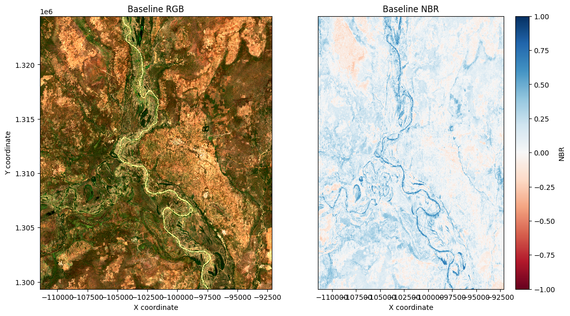
Visualiser le NBR
Pour voir comment le NBR correspond à une image standard, nous pouvons tracer les données NBR de base côte à côte avec un tracé RVB de la zone d’étude :
[13]:
# Set up subplots
f, (ax1, ax2) = plt.subplots(nrows=1, ncols=2, figsize=(13, 7))

# Visualise baseline image as true colour image
rgb(baseline_image,
    bands=['red', 'green', 'blue'],
    ax=ax1)
ax1.set_title('Baseline RGB')
ax1.set_xlabel('X coordinate')
ax1.set_ylabel('Y coordinate')

# Visualise baseline image as NBR image
baseline_NBR.plot(cmap='RdBu', vmin=-1, vmax=1, ax=ax2)
ax2.set_title('Baseline NBR')
ax2.yaxis.set_visible(False)
ax2.set_xlabel('X coordinate')

plt.show()
Charger les données post-incendie
Nous chargeons maintenant des images qui se produisent jusqu’à 30 jours après l’incendie. Étant donné que nous avons précédemment défini la zone d’intérêt et les mesures avec le paramètre « query », nous pouvons le réutiliser pour simplifier la commande de chargement, en notant que nous devons uniquement modifier la variable « time » pour utiliser les dates post-incendie calculées précédemment.
Veuillez être patient. Le chargement des données peut prendre quelques minutes et la progression sera indiquée par une sortie texte. Le chargement est terminé lorsque l’état de la cellule passe de « [*] » à « [numéro] ».
[14]:
# Load post-fire NRT data from Sentinel-2A and 2B
post_col =  load_ard(dc=dc,
                     products=products,
                     time=(start_date_post, end_date_post),
                     min_gooddata=min_gooddata,
                     output_crs=output_crs,
                     group_by='solar_day',
                     **query)
Using pixel quality parameters for Sentinel 2
Finding datasets
    s2_l2a_c1
Counting good quality pixels for each time step
Filtering to 5 out of 6 time steps with at least 60.0% good quality pixels
Applying pixel quality/cloud mask
Re-scaling Sentinel-2 C1 data
Loading 5 time steps
Découpez les ensembles de données selon la forme de la zone d’étude
[15]:
post_col = post_col.where(aoi_raster==1)
Générer un rapport de brûlure normalisé pour l’image post-incendie
Le code de la cellule suivante calcule le NBR pour la première image de l’ensemble de données post-incendie. Si l’image est très trouble, essayez une autre image en modifiant l’index dans post_col.isel(time=0). > Remarque : la valeur maximale de l’index est déterminée par le nombre d’images que vous avez chargées. Vérifiez le nombre d’intervalles de temps répertoriés ci-dessus dans la sortie load_ard pour l’ensemble de données post-incendie. Python compte à partir de 0, donc l’index maximal que vous pouvez utiliser sera inférieur d’un au nombre d’intervalles de temps.
Bien que la première image vous donne une image immédiate du paysage proche de l’incendie, vous pouvez également générer l’image médiane à partir de la période de 30 jours suivant l’incendie en utilisant le code ci-dessous. Si vous l’utilisez, commentez le code de l’image unique, puis copiez et collez le code de l’image médiane dans la cellule ci-dessous.
Médian
# Calculate NBR on all post-fire images
post_combined = calculate_indices(post_col, index='NBR', satellite_mission='s2', drop=False)

# Calculate the median post-fire image
post_image = post_combined.median(dim='time')

# Select NBR
post_NBR = post_image.NBR
post_NBR
[16]:
### Use a single image:

# Select the most recent image after the fire
post_image = post_col.isel(time=0)

# Calculate NBR
post_image = calculate_indices(post_image, index='NBR', satellite_mission='s2', drop=False)

# Select NBR
post_NBR = post_image.NBR
Données des points d’accès MODIS et VIIRS
Le système de gestion des ressources (FIRMS) fournit des informations sur les points chauds observés par satellite pour les incendies actifs en temps quasi réel (NRT) et les incendies historiques. Les informations sur les points chauds sont générées à la fois par le spectroradiomètre imageur à résolution moyenne (MODIS) et par la suite de radiomètres imageurs infrarouges visibles (VIIRS).
Ici, les données sur les points chauds du FIRMS sont utilisées pour analyser les changements du NBR aux emplacements identifiés comme des incendies actifs (ou historiques). Pour obtenir les données du FIRMS, une nouvelle demande peut être créée sur la page Web Archive Download. Il est possible de spécifier la région et les dates d’intérêt pour les informations sur les points chauds. Une fois le traitement de la demande terminé, les fichiers de formes contenant les données de MODIS C6 et VIIRS seront disponibles en téléchargement. Les fichiers de points chauds pour MODIS et VIIRS sont traités séparément.
Comme la région utilisée pour demander des points d’accès peut être différente de la région utilisée pour traiter les données Sentinel-2, les deux étapes suivantes peuvent être effectuées hors ligne ou dans le bloc-notes. Les deux étapes de prétraitement mentionnées ci-dessus sont les suivantes :
Données des points chauds de clip pour (
lon_range, lat_range)Fusionner les informations sur les points d’accès de MODIS et VIIRS
Après avoir découpé et fusionné les informations des hotspots, ouvrez le fichier de formes des hotspots à l’aide de la cellule suivante :
[17]:
# Extract contents of zip file

with ZipFile('../Supplementary_data/Burnt_area_mapping/fire_hotspots.zip') as spots:
    spots.extractall(path="../Supplementary_data/Burnt_area_mapping")
La cellule suivante projette les points chauds de la projection source ("EPSG:4326") vers la projection que nous utilisons pour les données Sentinel-2 (EPSG:6933). Ici, nous avons utilisé proj4 pour transformer les emplacements des points chauds de la source vers une projection souhaitée.
[18]:
# Read shapefile into a geopandas GeoDataFrame

fire_hotspots = gpd.read_file("../Supplementary_data/Burnt_area_mapping/fire_hotspots/clip_merged.shp")

# Extract the location of hotspots from the GeoDataFrame into a numpy.ndarray
spot_locs = fire_hotspots.to_crs(epsg=6933)
spot_locs = np.array([[item.x, item.y] for item in spot_locs.geometry.to_list()])
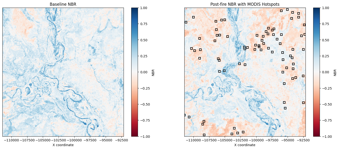
Examiner les points chauds
La cellule suivante trace les points chauds FIRMS sur l’image NBR post-incendie et trace l’image NBR de base à côté. Cela permet une comparaison directe des valeurs NBR avant et après l’incendie, ainsi que la corrélation spatiale des points chauds avec les zones enregistrées comme brûlées après l’incendie. Les points chauds sont représentés par des carrés noirs dans la deuxième image.
[19]:
fig, (ax1, ax2) = plt.subplots(nrows=1, ncols=2, figsize=(18, 7))

# Visualise baseline image as NBR image
baseline_NBR.plot(cmap='RdBu', vmin=-1, vmax=1, ax=ax1)
ax1.set_title('Baseline NBR')
ax1.yaxis.set_visible(False)
ax1.set_xlabel('X coordinate')

# Visualise post-fire image as NBR image and overplot hotspots
post_NBR.plot(cmap='RdBu', vmin=-1, vmax=1, ax=ax2)
ax2.plot(spot_locs[:,0], spot_locs[:,1], marker='s',
       linestyle='', mfc='None', mec='k', mew=1.5)
ax2.set_title('Post-fire NBR with MODIS Hotspots')
ax2.yaxis.set_visible(False)
ax2.set_xlabel('X coordinate');
Extraire les données aux points chauds du FIRMS pour le NBR de base et le NBR après incendie
L’étape suivante consiste à extraire les valeurs NBR aux emplacements des points chauds ; cette opération pour les images NBR de base et post-incendie nous permet d’examiner comment l’incendie a influencé les valeurs NBR.
Pour extraire les données, nous utilisons la méthode « xarray.DataArray.sel », qui renvoie un tableau bidimensionnel. Cela est dû à la manière dont nous avons spécifié les coordonnées des emplacements des points d’accès, qui sont un tableau numpy unidimensionnel. Les valeurs le long de la diagonale du tableau bidimensionnel renvoyé correspondent aux emplacements des points d’accès qui peuvent être obtenus à l’aide de la méthode « np.diagonal ».
[20]:
point_nbr = {}

# Extract baseline NBR at hotspot locations
point_nbr["baseline"] = np.diagonal(baseline_NBR.sel(x=spot_locs[:,0],
                                                     y=spot_locs[:,1],
                                                     method='nearest'))

# Extract post-fire NBR at hotspot locations
point_nbr["post"] = np.diagonal(post_NBR.sel(x=spot_locs[:,0],
                                             y=spot_locs[:,1],
                                             method='nearest'))
À l’aide des données extraites, nous pouvons créer un diagramme en boîte du NBR obtenu à partir des ensembles de données de base et post-incendie pour tous les emplacements des points chauds.
[21]:
ax = pd.DataFrame(point_nbr).boxplot(figsize=(10, 6), whis=0.75,
                                     patch_artist=True,
                                     vert=True, fontsize=14,
                                     return_type='both')

ax[0].set_ylabel("NBR", fontsize=14)
ax[0].set_title("NBR at FIRMS Hotspots", fontsize=14);
ax[0].set_xticklabels(["baseline", "post-fire"])
ax[0].grid(False)

colors = ['#addd8e', '#fdbb84']

for patch, color in zip(ax[1]['boxes'], colors):
    patch.set_facecolor(color)
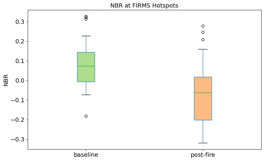
Ici, nous pouvons remarquer que le NBR post-incendie diminue par rapport au NBR de base aux points chauds, ce qui correspond au fait que ces endroits ont été touchés par l’incendie.
Nous pouvons également comparer l’évolution du NBR au cours de trois mois aux points chauds. Pour cela, nous utiliserons la méthode « xarray » pour extraire les données des emplacements des points chauds. Pour ce faire, nous extrayons également des versions nettoyées des dates des observations de base.
[22]:
# Get cleaned baseline observation dates
baseline_ard['time'] = baseline_ard.indexes['time'].normalize()
dates = (pd.to_datetime((baseline_ard.time).values)).strftime('%Y-%m-%d')

# Get the baseline NBR value for each image at all hotspots
baseline_nbr_spot = baseline_ard.NBR.sel(x=spot_locs[:,0],
                                         y=spot_locs[:,1],
                                         method='nearest')

nbr_over_time = {}
for i in range(len(dates)):
    nbr_over_time[dates[i]] = np.diagonal(baseline_nbr_spot[i,:,:])
nbr_over_time = pd.DataFrame(nbr_over_time)

# Create a box plot for each observation
ax = nbr_over_time.boxplot(figsize=(16, 4), whis=0.75,
                           patch_artist=True,
                           vert=True, return_type='both')
ax[0].set_ylabel("NBR", fontsize=14)
ax[0].set_title("NBR at MODIS Hotspots", fontsize=14);
ax[0].grid(False)

# Colour the boxes by the mean NBR of each observation
cm = plt.cm.get_cmap("Blues", len(nbr_over_time.index))
colors = [cm(item.get_ydata().mean()) for item in ax[1]['medians']]
for patch, color in zip(ax[1]['boxes'], colors):
    patch.set_facecolor(color)
ax[0].tick_params(axis='x', rotation=45)
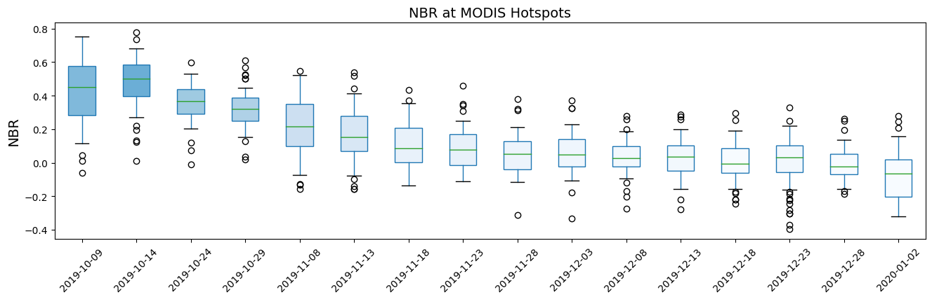
Après avoir tracé l’évolution du NBR sur une période de trois mois, nous pouvons remarquer qu’il y a une forte baisse du NBR entre octobre 2019 et novembre 2019, cependant, il y a peu ou pas de changement entre novembre 2019 et janvier 2020.
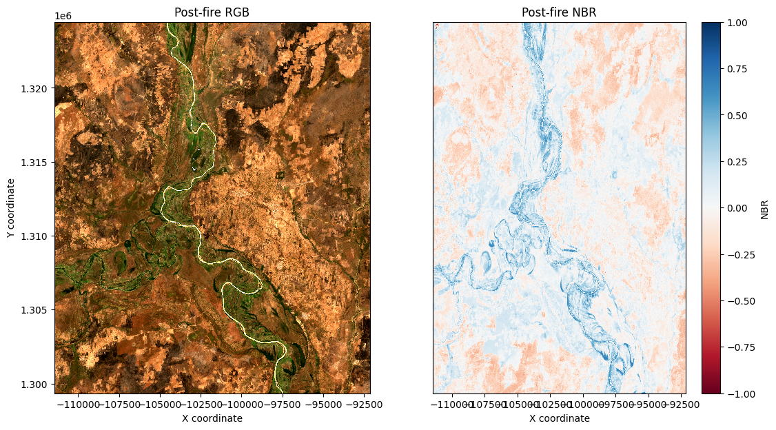
Enfin, nous traçons les données NBR post-incendie côte à côte avec un graphique RVB de la zone d’étude :
[23]:
# Set up subplots
f, (ax1, ax2) = plt.subplots(nrows=1, ncols=2, figsize=(13, 7))

# Visualise post-fire image as true colour image
rgb(post_image,
    bands=['red', 'green', 'blue'],
    ax=ax1)
ax1.set_title('Post-fire RGB')
ax1.set_xlabel('X coordinate')
ax1.set_ylabel('Y coordinate')

# Visualise post-fire image as NBR image
post_NBR.plot(cmap='RdBu', vmin=-1, vmax=1, ax=ax2)
ax2.set_title('Post-fire NBR')
ax2.yaxis.set_visible(False)
ax2.set_xlabel('X coordinate')

plt.show()
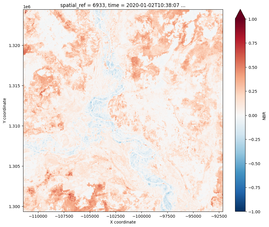
Calculer le rapport de combustion normalisé Delta
Nous pouvons maintenant calculer le delta NBR en soustrayant nos données NBR post-incendie de nos données NBR de base :
[24]:
delta_NBR = baseline_NBR - post_NBR

# Visualise dNBR image
delta_NBR.plot(cmap='RdBu_r', vmin=-1, vmax=1, figsize=(11, 9))
plt.xlabel('X coordinate')
plt.ylabel('Y coordinate')

plt.show()
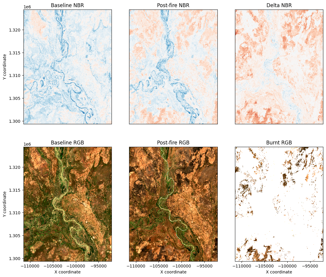
Appliquer le seuil au rapport de combustion normalisé Delta
Nous appliquons maintenant la valeur seuil dNBR pour essayer de réduire les faux positifs, en conservant uniquement les zones avec des valeurs dNBR supérieures à la valeur seuil choisie de 0,3. La valeur seuil choisie peut devoir être ajustée en fonction du cas d’utilisation.
[25]:
# Set threshold
threshold = 0.3

# Apply threshold
burnt = delta_NBR > threshold

# Mask post-fire true colour image
masked = delta_NBR.where(burnt==1)
Revisualisez les images en vraies couleurs avant et après incendie pour aider à ajuster le seuil NBR :
[26]:
# Set up subplots
f, axarr = plt.subplots(2, 3, figsize=(13, 11))
bands=['red', 'green', 'blue']

baseline_NBR.plot(cmap='RdBu', vmin=-1, vmax=1,
                  add_colorbar=False, ax=axarr[0, 0])
axarr[0, 0].set_title('Baseline NBR')
axarr[0, 0].set_ylabel('Y coordinate')
axarr[0, 0].xaxis.set_visible(False)

post_NBR.plot(cmap='RdBu', vmin=-1, vmax=1,
              add_colorbar=False, ax=axarr[0, 1])
axarr[0, 1].set_title('Post-fire NBR')
axarr[0, 1].yaxis.set_visible(False)
axarr[0, 1].xaxis.set_visible(False)

delta_NBR.plot(cmap='RdBu_r', vmin=-1, vmax=1,
               add_colorbar=False, ax=axarr[0, 2])
axarr[0, 2].set_title('Delta NBR')
axarr[0, 2].yaxis.set_visible(False)
axarr[0, 2].xaxis.set_visible(False)

rgb(baseline_image, bands=bands, ax=axarr[1, 0])
axarr[1, 0].set_title('Baseline RGB')
axarr[1, 0].set_title('Baseline RGB')
axarr[1, 0].set_xlabel('X coordinate')
axarr[1, 0].set_ylabel('Y coordinate')

rgb(post_image, bands=bands, ax=axarr[1,1])
axarr[1, 1].set_title('Post-fire RGB')
axarr[1, 1].set_xlabel('X coordinate')
axarr[1, 1].yaxis.set_visible(False)

rgb(post_image.where(burnt==1), bands=bands, ax=axarr[1, 2])
axarr[1, 2].set_title('Burnt RGB')
axarr[1, 2].set_xlabel('X coordinate')
axarr[1, 2].yaxis.set_visible(False)
Calculer la surface brûlée
La cellule suivante utilise la résolution des pixels Sentinel-2 pour estimer la quantité de surface brûlée, définie comme les zones dont les valeurs dNBR sont supérieures au seuil défini. Un certain nombre d’autres statistiques sont calculées, en tenant compte des zones qui ne contiennent aucune donnée.
[27]:
# Constants for calculating burnt area
pixel_length = resolution[1]  # in metres
m_per_km = 1000  # conversion from metres to kilometres

# Area per pixel
area_per_pixel = pixel_length ** 2 / m_per_km ** 2

# Calculate areas
unburnt_area = (delta_NBR <= threshold).sum() * area_per_pixel
burnt_area = burnt.sum() * area_per_pixel
not_nan_area = delta_NBR.notnull().sum() * area_per_pixel
nan_area = delta_NBR.isnull().sum() * area_per_pixel
total_area = unburnt_area + burnt_area + nan_area

print(f'Unburnt area:            {unburnt_area.item():.2f} km^2')
print(f'Burnt area:              {burnt_area.item():.2f} km^2')
print(f'Nan area:                {nan_area.item():.2f} km^2')
print(f'Total area (no nans):    {not_nan_area.item():.2f} km^2')
print(f'Total area (with nans):  {total_area.item():.2f} km^2')
print()
print(f'Percentage of total area burnt: {100*burnt_area.item()/total_area.item():.2f}%')
Unburnt area:            483.82 km^2
Burnt area:              0.81 km^2
Nan area:                0.44 km^2
Total area (no nans):    484.62 km^2
Total area (with nans):  485.07 km^2

Percentage of total area burnt: 0.17%
Exporter les résultats vers GeoTIFF
L’image de référence de base et l’image après incendie seront toutes deux enregistrées au format GeoTIFF multibande avec les bandes suivantes dans l’ordre suivant : Bleu, Vert, Rouge, NIR, SWIR.
L’image de la zone brûlée seuillée sera enregistrée sous forme d’image à bande unique, où une valeur de 1 = brûlée et une valeur de 0 = non brûlée.
[28]:
# Define an area name to be used in saved file names
area_name = 'Example'

# Write baseline reference image to multi-band GeoTIFF, overwriting if exists
write_cog(baseline_image.to_array(), f'{area_name}_baseline_image.tif', overwrite=True)

# Write post fire image to multi-band GeoTIFF, overwriting if exists
write_cog(post_image.to_array(), f'{area_name}_post_fire_image.tif', overwrite=True)

# Turn delta NBR into a Xarray Dataset for export to GeoTIFF
dnbr_dataset = delta_NBR.to_dataset(name='burnt_area')
# Write delta NBR to GeoTIFF, overwriting if exists
write_cog(dnbr_dataset.to_array(), f'{area_name}_delta_NBR.tif', overwrite=True)
[28]:
PosixPath('Example_delta_NBR.tif')
Informations Complémentaires
Licence Le code de ce notebook est sous licence Apache, version 2.0 <https://www.apache.org/licenses/LICENSE-2.0>`__.
Les données de Digital Earth Africa sont sous licence Creative Commons Attribution 4.0 <https://creativecommons.org/licenses/by/4.0/>.
Contact Si vous avez besoin d’aide, veuillez poster une question sur le canal Slack DE Africa <https://digitalearthafrica.slack.com/> ou sur le GIS Stack Exchange <https://gis.stackexchange.com/questions/ask?tags=open-data-cube> en utilisant la balise open-data-cube (vous pouvez consulter les questions posées précédemment `ici <https://gis.stackexchange.com/questions/tagged/open-data-
Si vous souhaitez signaler un problème avec ce notebook, vous pouvez en déposer un sur Github.
Version de Datacube compatible
[29]:
print(datacube.__version__)
1.8.20
Dernier test :
[30]:
from datetime import datetime
datetime.today().strftime('%Y-%m-%d')
[30]:
'2025-06-04'