Utilisation de « load_ard » pour charger et masquer plusieurs capteurs satellites
Mots-clés données utilisées ; landsat 5, données utilisées ; landsat 7, données utilisées ; landsat 8, données utilisées ; landsat 9, données utilisées ; sentinel-2, masquage des nuages, filtrage des nuages, qualité des pixels, dask
Description
Ce bloc-notes montre comment utiliser la fonction « load_ard » pour importer une série chronologique d’observations sans nuages sur l’Afrique à partir de plusieurs satellites Landsat (c’est-à-dire Landsat 5, 7, 8 et 9) et Sentinel-2 (c’est-à-dire Sentinel-2A et Sentinel-2B). La fonction applique automatiquement un masquage des nuages aux données d’entrée et renvoie toutes les données disponibles provenant de plusieurs capteurs sous la forme d’un seul « xarray.Dataset » combiné.
En option, la fonction peut être utilisée pour renvoyer uniquement les observations contenant une proportion minimale de pixels de bonne qualité, non nuageux ou ombragés. Cela peut être utilisé pour extraire des séries chronologiques visuellement attrayantes d’observations qui ne sont pas affectées par les nuages.
La fonction « load_ard » prend actuellement en charge les produits suivants :
Collection USGS 2 : « ls5_sr, ls7_sr, ls8_sr, ls9_sr »
Sentinelle 2 : « s2_l2a »
Sentinelle 1 : « s1_rtc »
Ce notebook montre comment utiliser « load_ard » pour
Chargez et combinez les données Landsat 5, 7, 8 et 9 dans un seul « xarray.Dataset »
Appliquez éventuellement un masque de nuage aux données résultantes
Filtrer les données résultantes pour ne conserver que les observations sans nuages
Application du traitement morphologique sur le masque de nuages
Filtrer les données avant le chargement à l’aide d’une fonction personnalisée
Charger les données Sentinel-2
Charger des données en mode paresseux à l’aide de Dask
Commencer
Pour exécuter cette analyse, exécutez toutes les cellules du bloc-notes, en commençant par la cellule « Charger les packages ».
Charger des paquets
[1]:
%matplotlib inline

import datacube
import matplotlib.pyplot as plt

from deafrica_tools.datahandling import load_ard
from deafrica_tools.plotting import rgb
Se connecter au datacube
[2]:
# Connect to datacube
dc = datacube.Datacube(app='Using_load_ard')
Chargement de plusieurs capteurs Landsat
La fonction load_ard peut être utilisée pour charger une seule série temporelle combinée de données masquées par des nuages provenant de plusieurs satellites Landsat. Dans sa forme la plus simple, vous pouvez utiliser la fonction de la même manière que dc.load en passant un ensemble de paramètres de requête spatiotemporels (par exemple, x, y, time, measurements, output_crs, resolution, group_by etc) directement dans la fonction (consultez la documentation dc.load pour toutes les options possibles). La principale différence avec dc.load est que la fonction nécessite également un objet Datacube existant, qui est passé à l’aide du paramètre dc. Cela nous donne la flexibilité de charger des données à partir de cubes de données de développement ou expérimentaux.
Dans les exemples ci-dessous, nous chargeons trois bandes de données (« rouge », « vert », « bleu ») à partir des trois produits USGS Collection 2 (Landsat 5, 7, 8 et 9) en spécifiant :
produits=['ls5_sr', 'ls7_sr', 'ls8_sr', ls9_sr']
Remarque : « load_ard » présente certaines limitations en raison de sa conception. Une partie importante de sa fonctionnalité prévue est de fournir un moyen simple de concaténer Landsat 5, 7, 8 et 9 ensemble pour former un seul objet xarray. Cependant, cela signifie que « load_ard » ne peut appliquer un masquage de qualité de pixel qu’aux catégories pq qui sont communes à tous les capteurs Landsat. Par exemple, Landsat-8 dispose d’un indicateur de bits dédié pour les bandes de cirrus, mais Landsat 5 et 7 ne l’ont pas. Cela signifie que « load_ard » ne peut pas accepter « cirrus » : « high_confidence » comme catégorie pq. Le même problème s’applique également au masquage des aérosols, Landat 5 et 7 ont des moyens différents d’enregistrer les aérosols à forte concentration que Landsat 8, et donc « load_ard » ne prend pas en charge le masquage des aérosols.
La fonction génère le nombre d’observations pour chaque produit et le nombre total chargé si le paramètre « verbose= » est défini sur « True » (ce qui est le cas par défaut).
Syntaxe explicite
L’exemple suivant montre comment les paramètres clés peuvent être transmis directement à « load_ard ».
[3]:
ds = load_ard(dc=dc,
              products=['ls5_sr',
                        'ls7_sr',
                        'ls8_sr',
                        'ls9_sr'],
              x=(-16.45, -16.6),
              y=(13.675, 13.8),
              time=('2021-09', '2021-12'),
              measurements = ['red','green','blue'],
              output_crs='epsg:6933',
              resolution=(-30, 30),
              group_by='solar_day')

print(ds)
Using pixel quality parameters for USGS Collection 2
Finding datasets
    ls5_sr
    ls7_sr
    ls8_sr
    ls9_sr
Applying pixel quality/cloud mask
Re-scaling Landsat C2 data
Loading 17 time steps
/usr/local/lib/python3.10/dist-packages/rasterio/warp.py:344: NotGeoreferencedWarning: Dataset has no geotransform, gcps, or rpcs. The identity matrix will be returned.
  _reproject(
<xarray.Dataset>
Dimensions:      (time: 17, y: 517, x: 484)
Coordinates:
  * time         (time) datetime64[ns] 2021-09-05T11:27:43.160264 ... 2021-12...
  * y            (y) float64 1.744e+06 1.744e+06 ... 1.729e+06 1.728e+06
  * x            (x) float64 -1.602e+06 -1.602e+06 ... -1.587e+06 -1.587e+06
    spatial_ref  int32 6933
Data variables:
    red          (time, y, x) float32 nan nan nan nan nan ... nan nan nan nan
    green        (time, y, x) float32 nan nan nan nan nan ... nan nan nan nan
    blue         (time, y, x) float32 nan nan nan nan nan ... nan nan nan nan
Attributes:
    crs:           epsg:6933
    grid_mapping:  spatial_ref
Syntaxe de la requête
L’exemple suivant montre comment les paramètres clés peuvent être stockés dans un dictionnaire « query », pour être transmis comme paramètre unique à « load_ard ». La « query » peut ensuite être réutilisée dans d’autres appels à « load_ard ».
[4]:
# Create a reusable query
query = {
    'x': (-16.45, -16.6),
    'y': (13.675, 13.8),
    'time': ('2021-09', '2021-12'),
    'measurements': ['red', 'green', 'blue'],
    'group_by': 'solar_day',
    'output_crs' : 'epsg:6933',
}
[5]:
# Load available data from all three Landsat satellites
ds = load_ard(dc=dc,
              products=['ls5_sr',
                        'ls7_sr',
                        'ls8_sr',
                        'ls9_sr'],
              resolution=(-30, 30),
              **query)

# Print output data
print(ds)
Using pixel quality parameters for USGS Collection 2
Finding datasets
    ls5_sr
    ls7_sr
    ls8_sr
    ls9_sr
Applying pixel quality/cloud mask
Re-scaling Landsat C2 data
Loading 17 time steps
<xarray.Dataset>
Dimensions:      (time: 17, y: 517, x: 484)
Coordinates:
  * time         (time) datetime64[ns] 2021-09-05T11:27:43.160264 ... 2021-12...
  * y            (y) float64 1.744e+06 1.744e+06 ... 1.729e+06 1.728e+06
  * x            (x) float64 -1.602e+06 -1.602e+06 ... -1.587e+06 -1.587e+06
    spatial_ref  int32 6933
Data variables:
    red          (time, y, x) float32 nan nan nan nan nan ... nan nan nan nan
    green        (time, y, x) float32 nan nan nan nan nan ... nan nan nan nan
    blue         (time, y, x) float32 nan nan nan nan nan ... nan nan nan nan
Attributes:
    crs:           epsg:6933
    grid_mapping:  spatial_ref
Travailler avec le masquage des nuages
En traçant une tranche de temps à partir des données que nous avons chargées ci-dessus, vous pouvez voir une zone de pixels blancs où les nuages ont été masqués et définis sur « NaN » :
[6]:
# Plot single observation
rgb(ds, col='time', col_wrap=6)
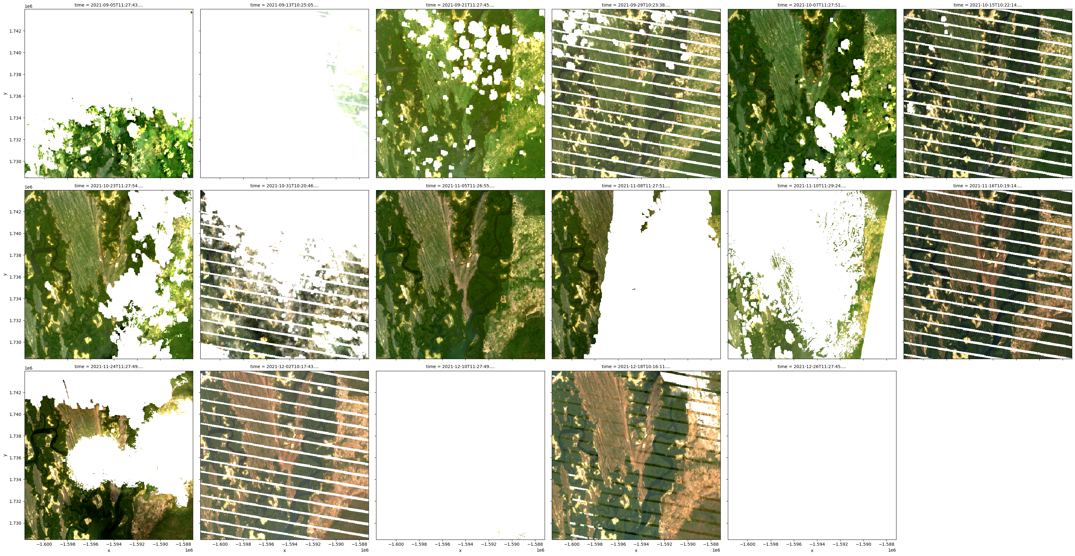
Par défaut, « load_ard » applique un masque de qualité de pixel aux données chargées en utilisant la bande de qualité de pixel du capteur.
Pour la collection USGS 2, les paramètres de masque suivants sont appliqués à la bande « qa_pixel » :
{
'cloud':"high_confidence",
'cloud_shadow':"high_confidence",
'nodata':True
}
Pour Sentinel 2, les paramètres de masque suivants sont appliqués à la bande SCL :
[
"cloud high probability",
"cloud medium probability",
"thin cirrus",
"cloud shadows",
"saturated or defective",
"no data"
]
Remarque : ces paramètres de masquage peuvent être personnalisés à l’aide du paramètre « categories_to_mask_ls » pour les données USGS et du paramètre « categories_to_mask_s2 » pour les données Sentinel 2
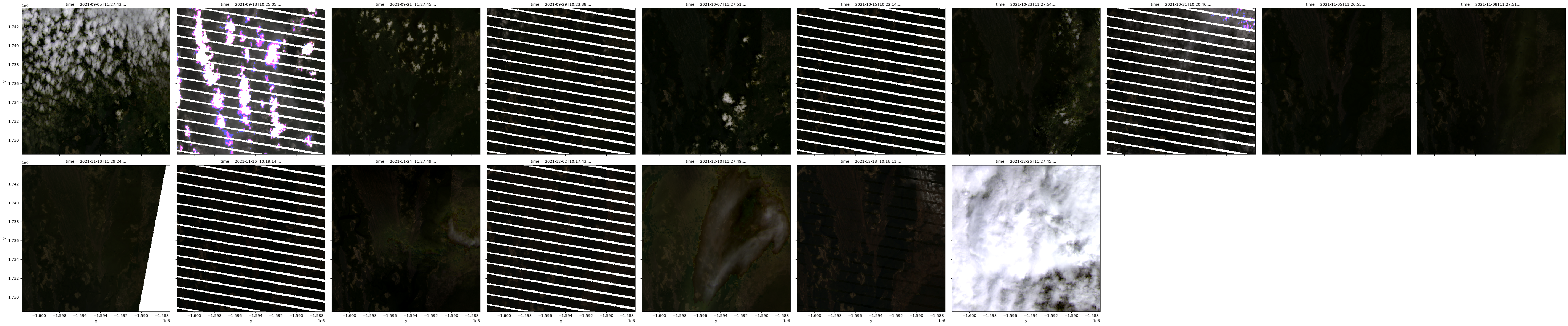
Nous pouvons désactiver complètement le masquage des pixels en définissant « mask_pixel_quality=False » :
[7]:
# Load available data with cloud masking deactivated
ds = load_ard(dc=dc,
              products=['ls5_sr',
                        'ls7_sr',
                        'ls8_sr',
                        'ls9_sr'],
              mask_pixel_quality=False,
              resolution=(-30, 30),
              **query)

# Plot single observation
rgb(ds, col='time', col_wrap=10)
Using pixel quality parameters for USGS Collection 2
Finding datasets
    ls5_sr
    ls7_sr
    ls8_sr
    ls9_sr
Re-scaling Landsat C2 data
Loading 17 time steps
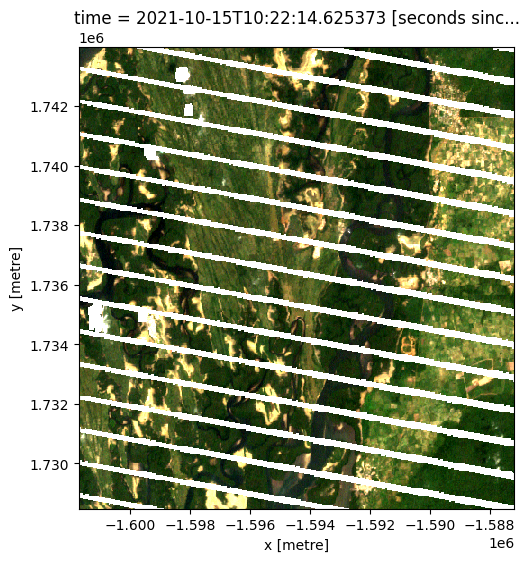
Filtrage des observations non nuageuses
En plus de masquer les nuages, « load_ard » vous permet de supprimer toute observation satellite contenant moins qu’une proportion minimale de pixels de bonne qualité (par exemple, non nuageux). Cela peut être utilisé pour obtenir une série temporelle contenant uniquement des observations claires et sans nuages.
Pour ignorer toutes les observations avec moins de « X % de pixels de bonne qualité », utilisez le paramètre « min_gooddata ». Par exemple, « min_gooddata=0.90 » renverra uniquement les observations où moins de 10 % des pixels contiennent des nuages, des ombres de nuages ou d’autres données non valides, ce qui entraînera un nombre plus réduit d’images claires et sans nuages renvoyées par la fonction :
[8]:
# Load available data filtered to 90% clear observations
ds = load_ard(dc=dc,
              products=['ls5_sr',
                        'ls7_sr',
                        'ls8_sr',
                        'ls9_sr'],
              min_gooddata=0.90,
              resolution=(-30, 30),
              **query)

# Plot single observation
rgb(ds, index=2)
Using pixel quality parameters for USGS Collection 2
Finding datasets
    ls5_sr
    ls7_sr
    ls8_sr
    ls9_sr
Counting good quality pixels for each time step
Filtering to 7 out of 17 time steps with at least 90.0% good quality pixels
Applying pixel quality/cloud mask
Re-scaling Landsat C2 data
Loading 7 time steps
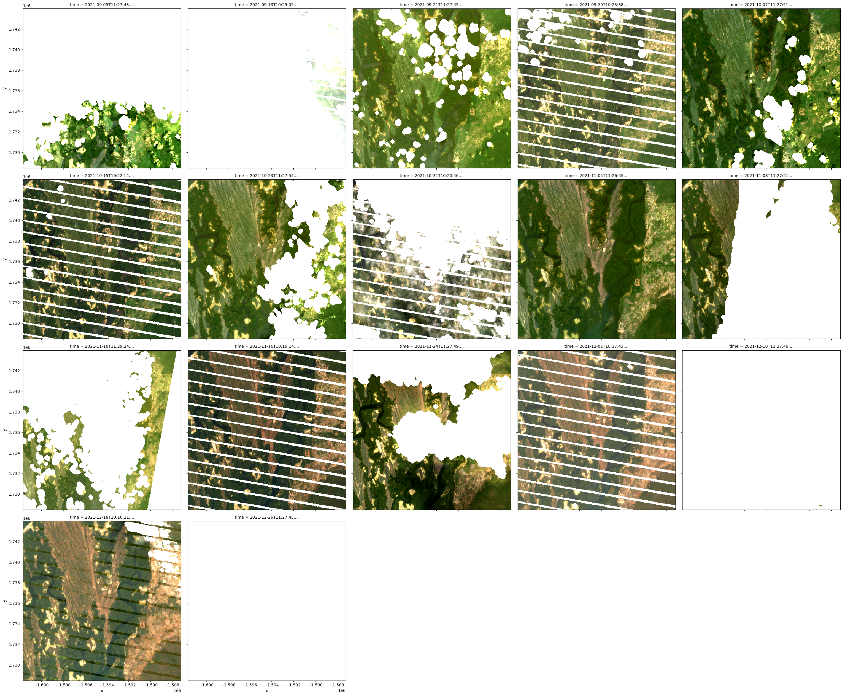
Application du traitement morphologique sur le masque de nuages
Les algorithmes de masquage des nuages employés par Sentinel-2 et Landsat présentent des limites connues importantes. Par exemple, les objets brillants comme les bâtiments et les côtes sont souvent confondus avec des nuages. Nous pouvons améliorer les faux positifs détectés par le masque de qualité des pixels de Landsat et Sentinel-2 en appliquant des techniques de traitement d’images morphologiques binaires (par exemple, binary_closing, binary_erosion etc.). La bibliothèque Open-Data-Cube odc-algo possède une fonction, odc.algo.mask_cleanup qui peut effectuer quelques-unes de ces opérations. Ci-dessous, nous allons essayer d’améliorer le masque de nuage en appliquant un certain nombre de ces filtres.
N’hésitez pas à expérimenter avec les valeurs dans « filtres »
[9]:
# set the filters to apply
filters = filters = [("opening", 4),("dilation", 2)]

# # Load data
data = load_ard(dc=dc,
              products=['ls5_sr',
                        'ls7_sr',
                        'ls8_sr',
                        'ls9_sr'],
              resolution=(-30, 30),
              mask_filters=filters,
              **query)
Using pixel quality parameters for USGS Collection 2
Finding datasets
    ls5_sr
    ls7_sr
    ls8_sr
    ls9_sr
Applying morphological filters to pq mask [('opening', 4), ('dilation', 2)]
Applying pixel quality/cloud mask
Re-scaling Landsat C2 data
Loading 17 time steps
Ci-dessous, vous remarquerez peut-être que dans les deuxième et quatrième images, certains des faux positifs sur la rivière/les berges ont été supprimés par les filtres morphologiques
[10]:
# plot the data
rgb(data, col="time", col_wrap=5)
Filtrage des données avant le chargement à l’aide d’une fonction personnalisée
La fonction « load_ard » possède un paramètre de prédicat puissant qui vous permet de filtrer les observations satellite avant qu’elles ne soient réellement chargées à l’aide d’une fonction personnalisée. Voici quelques exemples de cas où cela peut être utile :
Filtrage pour renvoyer les données d’une saison spécifique (par exemple, été, hiver)
Filtrage pour renvoyer les données acquises un jour particulier de l’année
Filtrage pour renvoyer des données basées sur un ensemble de données externe (par exemple, des données acquises lors de conditions climatiques spécifiques telles qu’une sécheresse ou une inondation)
Une fonction de prédicat doit prendre un objet « datacube.model.Dataset » comme entrée (par exemple, tel que renvoyé par « dc.find_datasets(product=”ls8_sr”, **query)[0] ») et renvoyer soit « True » soit « False ». Par exemple, une fonction de prédicat peut être utilisée pour renvoyer True uniquement pour les ensembles de données acquis en avril :
dataset.time.begin.month == 4
Filtrer sur un seul mois
Dans l’exemple ci-dessous, nous créons une fonction de prédicat simple qui filtrera nos données pour renvoyer uniquement les données satellite acquises en avril :
[11]:
def filter_april(dataset):
    return dataset.time.begin.month == 4

# Load data that passes the `filter_april` function
ds = load_ard(dc=dc,
             products=['ls5_sr',
                        'ls7_sr',
                        'ls8_sr'],
              x=(-16.45, -16.6),
              y=(13.675, 13.8),
              time=('2016', '2018'),
              measurements = ['red', 'green', 'blue'],
              output_crs='epsg:6933',
              predicate=filter_april,
              resolution=(-30, 30),
              group_by='solar_day')

# Print output data
print(ds)
Using pixel quality parameters for USGS Collection 2
Finding datasets
    ls5_sr
    ls7_sr
    ls8_sr
Filtering datasets using filter function
Applying pixel quality/cloud mask
Re-scaling Landsat C2 data
Loading 10 time steps
<xarray.Dataset>
Dimensions:      (time: 10, y: 517, x: 484)
Coordinates:
  * time         (time) datetime64[ns] 2016-04-16T11:27:02.825796 ... 2018-04...
  * y            (y) float64 1.744e+06 1.744e+06 ... 1.729e+06 1.728e+06
  * x            (x) float64 -1.602e+06 -1.602e+06 ... -1.587e+06 -1.587e+06
    spatial_ref  int32 6933
Data variables:
    red          (time, y, x) float32 0.0824 0.08374 0.08391 ... 0.1524 0.15
    green        (time, y, x) float32 0.08861 0.08985 0.09015 ... 0.1053 0.1001
    blue         (time, y, x) float32 0.06472 0.06551 0.06568 ... 0.0665 0.06414
Attributes:
    crs:           epsg:6933
    grid_mapping:  spatial_ref
Nous pouvons imprimer les pas de temps renvoyés par load_ard pour vérifier qu’ils incluent désormais uniquement les observations d’avril (par exemple 2018-04-…) :
[12]:
ds.time.values
[12]:
array(['2016-04-16T11:27:02.825796000', '2016-04-24T11:29:48.253992000',
       '2017-04-03T11:27:01.738770000', '2017-04-11T11:29:47.043543000',
       '2017-04-19T11:26:52.881313000', '2017-04-27T11:29:53.632066000',
       '2018-04-06T11:26:52.293262000', '2018-04-14T11:28:13.576859000',
       '2018-04-22T11:26:42.800959000', '2018-04-30T11:27:56.435231000'],
      dtype='datetime64[ns]')
Filtrer sur une seule saison
Un exemple de fonction de prédicat qui renverra des données d’une saison d’intérêt ressemblerait à ceci :
def seasonal_filter(dataset, season=[12,1,2]):
        #return true if month is in defined season
        return dataset.time.begin.month in season
Après avoir appliqué cette fonction de prédicat, l’exécution de la commande suivante démontre que notre ensemble de données ne contient que des mois pendant la période de décembre, janvier et février
ds.time.dt.season :

<xarray.DataArray 'season' (time: 37)>
array(['DJF', 'DJF', 'DJF', 'DJF', 'DJF', 'DJF', 'DJF', 'DJF', 'DJF',
       'DJF', 'DJF', 'DJF', 'DJF', 'DJF', 'DJF', 'DJF', 'DJF', 'DJF',
       'DJF', 'DJF', 'DJF', 'DJF', 'DJF', 'DJF', 'DJF', 'DJF', 'DJF',
       'DJF', 'DJF', 'DJF', 'DJF', 'DJF', 'DJF', 'DJF', 'DJF', 'DJF',
       'DJF'], dtype='<U3')
Coordinates:
  * time     (time) datetime64[ns] 2016-01-05T10:27:44.213284 ... 2017-12-26T10:23:43.129624
Chargement des données Sentinel-2
Les données des satellites Sentinel-2A et Sentinel-2B peuvent également être chargées à l’aide de « load_ard ». Pour ce faire, nous devons spécifier le produit Sentinel-2 (['s2a_l2a'] - les deux capteurs S2a et S2b sont couverts par ce nom de produit) à la place des produits Landsat ci-dessus.
[13]:
# Load available data from S2
s2 = load_ard(dc=dc,
              products=['s2_l2a'],
              resolution=(-20, 20),
              **query)

# # Print output data
print(s2)
Using pixel quality parameters for Sentinel 2
Finding datasets
    s2_l2a
Applying pixel quality/cloud mask
Loading 24 time steps
<xarray.Dataset>
Dimensions:      (time: 24, y: 776, x: 724)
Coordinates:
  * time         (time) datetime64[ns] 2021-09-04T11:47:39 ... 2021-12-28T11:...
  * y            (y) float64 1.744e+06 1.744e+06 ... 1.729e+06 1.728e+06
  * x            (x) float64 -1.602e+06 -1.602e+06 ... -1.587e+06 -1.587e+06
    spatial_ref  int32 6933
Data variables:
    red          (time, y, x) float32 1.062e+03 1.08e+03 ... 348.0 373.0
    green        (time, y, x) float32 1.184e+03 1.28e+03 ... 354.0 340.0
    blue         (time, y, x) float32 1.264e+03 1.346e+03 ... 119.0 136.0
Attributes:
    crs:           epsg:6933
    grid_mapping:  spatial_ref
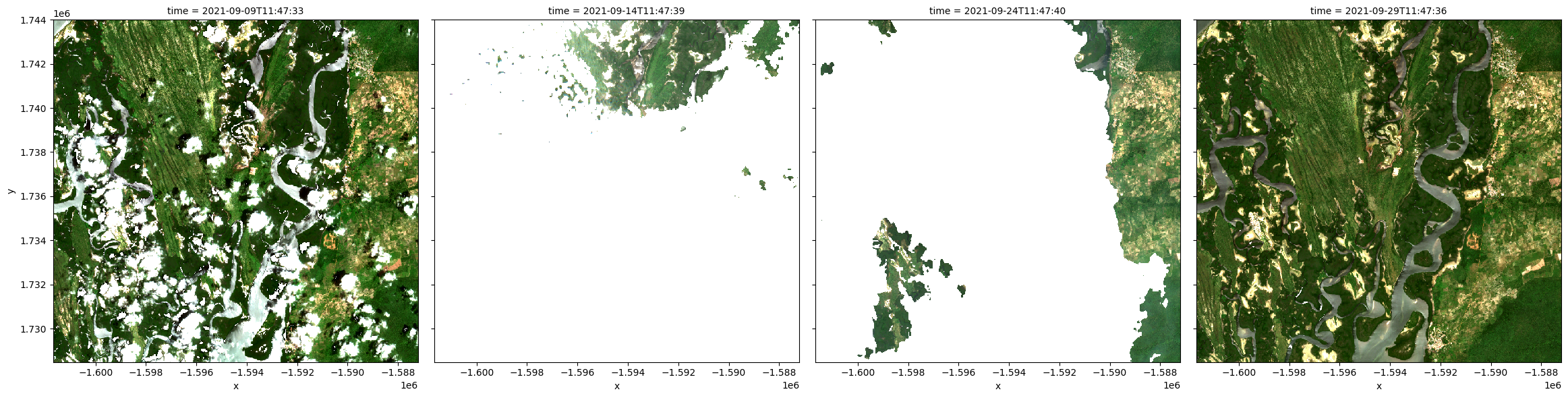
Les pixels nuageux sont masqués par défaut dans les observations résultantes, de la même manière que Landsat
[14]:
# Plot single observation
rgb(s2, index=[1,2,4,5])
Chargement paresseux avec Dask
Au lieu de charger les données directement (ce qui peut prendre beaucoup de temps et nécessiter de grandes quantités de mémoire), toutes les données du Datacube peuvent être chargées de manière différée à l’aide de Dask. Cette approche peut être très utile lorsque vous devez charger de grandes quantités de données sans faire planter votre analyse, ou si vous souhaitez ensuite faire évoluer votre analyse en répartissant les tâches en parallèle sur plusieurs travailleurs.
La fonction load_ard peut être facilement adaptée pour charger les données de manière paresseuse plutôt que de les charger en mémoire en fournissant un paramètre dask_chunks en utilisant soit la syntaxe explicite, soit la syntaxe de requête. Le minimum requis pour charger les données de manière paresseuse est dask_chunks={}, mais le découpage peut également être effectué spatialement (par exemple dask_chunks={'x': 3000, 'y': 3000}) ou par temps (par exemple dask_chunks={'time': 1}) en fonction de l’analyse effectuée. Consultez la documentation Dask pour plus d’informations sur la définition des tailles de bloc.
Pour en savoir plus sur le chargement différé avec Dask, consultez le Dask notebook.
[15]:
# Load available data from both S2 datasets
s2 = load_ard(dc=dc,
              products=['s2_l2a'],
              resolution=(-20, 20),
              dask_chunks={'time':1,'x':500,'y':500},
              **query)

# Print output data
print(s2)
Using pixel quality parameters for Sentinel 2
Finding datasets
    s2_l2a
Applying pixel quality/cloud mask
Returning 24 time steps as a dask array
<xarray.Dataset>
Dimensions:      (time: 24, y: 776, x: 724)
Coordinates:
  * time         (time) datetime64[ns] 2021-09-04T11:47:39 ... 2021-12-28T11:...
  * y            (y) float64 1.744e+06 1.744e+06 ... 1.729e+06 1.728e+06
  * x            (x) float64 -1.602e+06 -1.602e+06 ... -1.587e+06 -1.587e+06
    spatial_ref  int32 6933
Data variables:
    red          (time, y, x) float32 dask.array<chunksize=(1, 500, 500), meta=np.ndarray>
    green        (time, y, x) float32 dask.array<chunksize=(1, 500, 500), meta=np.ndarray>
    blue         (time, y, x) float32 dask.array<chunksize=(1, 500, 500), meta=np.ndarray>
Attributes:
    crs:           epsg:6933
    grid_mapping:  spatial_ref
Informations Complémentaires
Licence : Le code de ce carnet est sous licence Apache, version 2.0 <https://www.apache.org/licenses/LICENSE-2.0>. Les données de Digital Earth Africa sont sous licence Creative Commons par attribution 4.0 <https://creativecommons.org/licenses/by/4.0/>.
Contact : Si vous avez besoin d’aide, veuillez poster une question sur le canal Slack Open Data Cube <http://slack.opendatacube.org/>`__ ou sur le GIS Stack Exchange en utilisant la balise open-data-cube (vous pouvez consulter les questions posées précédemment ici). Si vous souhaitez signaler un problème avec ce bloc-notes, vous pouvez en déposer un sur Github.
Version de Datacube compatible :
[16]:
print(datacube.__version__)
1.8.15
Dernier test :
[17]:
from datetime import datetime
datetime.today().strftime('%Y-%m-%d')
[17]:
'2023-08-14'