Calcul des indices de bande

Produits utilisés : s2_l2a

Mots clés données utilisées ; sentinel-2, indice de bande ; NDVI, indice de bande ; NDWI, indice de bande ; MNDWI

Aperçu

Les indices de télédétection sont des combinaisons de bandes spectrales utilisées pour mettre en évidence les caractéristiques des données et du paysage sous-jacent. Par exemple, l’un des indices les plus couramment utilisés est l’indice de végétation par différence normalisée (NDVI), qui utilise le rapport entre la bande rouge et la bande proche infrarouge (NIR) pour mettre en évidence la végétation saine (voir ici pour une explication plus approfondie). En utilisant les archives de données satellite prêtes à l’analyse de Digital Earth Africa, nous pouvons facilement calculer une large gamme d’indices de télédétection qui peuvent être utilisés pour aider à cartographier et à surveiller des caractéristiques telles que la végétation et l’eau de manière cohérente dans le temps, ou comme entrées pour l’apprentissage automatique ou les algorithmes de classification.

Description

Ce cahier montre comment :

Calculer un index manuellement à l’aide de « xarray »
Calculer un ou plusieurs indices à l’aide de la fonction calculate_indices de deafrica_bandindices.py

Commencer

Pour exécuter cette analyse, exécutez toutes les cellules du bloc-notes, en commençant par la cellule « Charger les packages ».

Charger des paquets

[1]:

%matplotlib inline

import datacube
import matplotlib.pyplot as plt
import xarray as xr
import geopandas as gpd
from odc.geo.geom import Geometry

from deafrica_tools.datahandling import load_ard, mostcommon_crs
from deafrica_tools.plotting import rgb
from deafrica_tools.bandindices import calculate_indices
from deafrica_tools.areaofinterest import define_area

Se connecter au datacube

[2]:

dc = datacube.Datacube(app='Calculating_band_indices')

Créer une requête et charger des données satellite

Pour démontrer comment calculer un indice de télédétection, nous devons d’abord charger une série chronologique de données satellite pour une zone. Nous utiliserons les données du satellite Sentinel-2 :

Pour définir la zone d’intérêt, deux méthodes sont disponibles :

En spécifiant la latitude, la longitude et la zone tampon. Cette méthode nécessite que vous saisissiez la latitude centrale, la longitude centrale et la valeur de la zone tampon en degrés carrés autour du point central que vous souhaitez analyser. Par exemple, « lat = 10,338 », « lon = -1,055 » et « buffer = 0,1 » sélectionneront une zone avec un rayon de 0,1 degré carré autour du point avec les coordonnées (10,338, -1,055).
By uploading a polygon as a GeoJSON or Esri Shapefile. If you choose this option, you will need to upload the geojson or ESRI shapefile into the Sandbox using Upload Files button in the top left corner of the Jupyter Notebook interface. ESRI shapefiles must be uploaded with all the related files (.cpg, .dbf, .shp, .shx). Once uploaded, you can use the shapefile or geojson to define the area of interest. Remember to update the code to call the file you have uploaded.

Pour utiliser l’une de ces méthodes, vous pouvez décommenter la ligne de code concernée et commenter l’autre. Pour commenter une ligne, ajoutez le symbole "#" avant le code que vous souhaitez commenter. Par défaut, la première option qui définit l’emplacement à l’aide de la latitude, de la longitude et du tampon est utilisée.

Si vous exécutez le bloc-notes pour la première fois, conservez les paramètres par défaut ci-dessous. Cela permettra de démontrer le fonctionnement de l’analyse et de fournir des résultats significatifs.

[3]:

# Method 1: Specify the latitude, longitude, and buffer
aoi = define_area(lat=13.94, lon=-16.54, buffer=0.125)

# Method 2: Use a polygon as a GeoJSON or Esri Shapefile.
# aoi = define_area(vector_path='aoi.shp')

#Create a geopolygon and geodataframe of the area of interest
geopolygon = Geometry(aoi["features"][0]["geometry"], crs="epsg:4326")
geopolygon_gdf = gpd.GeoDataFrame(geometry=[geopolygon], crs=geopolygon.crs)

# Get the latitude and longitude range of the geopolygon
lat_range = (geopolygon_gdf.total_bounds[1], geopolygon_gdf.total_bounds[3])
lon_range = (geopolygon_gdf.total_bounds[0], geopolygon_gdf.total_bounds[2])

# Create a reusable query
query = {
    'x': lon_range,
    'y': lat_range,
    'time': ('2019-06', '2020-06'),
    'resolution': (-30, 30)
}

# Identify the most common projection system in the input query
output_crs = mostcommon_crs(dc=dc, product='s2_l2a', query=query)

# Load available data from Sentinel-2 and filter to retain only times
# with at least 99% good data
ds = load_ard(dc=dc,
              products=['s2_l2a'],
              min_gooddata=0.99,
              measurements=['red', 'green', 'blue', 'swir_1', 'swir_2', 'nir', 'nir_2'],
              output_crs=output_crs,
              **query)

Using pixel quality parameters for Sentinel 2
Finding datasets
    s2_l2a
Counting good quality pixels for each time step

/opt/venv/lib/python3.12/site-packages/rasterio/warp.py:385: NotGeoreferencedWarning: Dataset has no geotransform, gcps, or rpcs. The identity matrix will be returned.
  dest = _reproject(

Filtering to 16 out of 78 time steps with at least 99.0% good quality pixels
Applying pixel quality/cloud mask
Loading 16 time steps

Il est fortement recommandé de charger les données avec « load_ard » lors du calcul des indices et lors de l’utilisation de la fonction « calculate_indices » présentée ci-dessous. En effet, « load_ard » effectue le nettoyage et la mise à l’échelle des données nécessaires pour des résultats d’index plus robustes.

[4]:

print(ds)

<xarray.Dataset> Size: 378MB
Dimensions:      (time: 16, y: 929, x: 908)
Coordinates:
  * time         (time) datetime64[ns] 128B 2019-07-07T11:47:42 ... 2020-05-1...
  * y            (y) float64 7kB 1.556e+06 1.556e+06 ... 1.528e+06 1.528e+06
  * x            (x) float64 7kB 3.2e+05 3.201e+05 ... 3.472e+05 3.472e+05
    spatial_ref  int32 4B 32628
Data variables:
    red          (time, y, x) float32 54MB 2.965e+03 2.463e+03 ... nan nan
    green        (time, y, x) float32 54MB 2.132e+03 1.751e+03 ... nan nan
    blue         (time, y, x) float32 54MB 1.119e+03 921.0 1.285e+03 ... nan nan
    swir_1       (time, y, x) float32 54MB 5.63e+03 5.547e+03 ... nan nan
    swir_2       (time, y, x) float32 54MB 5.131e+03 4.916e+03 ... nan nan
    nir          (time, y, x) float32 54MB 4.045e+03 3.745e+03 ... nan nan
    nir_2        (time, y, x) float32 54MB 4.177e+03 4.228e+03 ... nan nan
Attributes:
    crs:           EPSG:32628
    grid_mapping:  spatial_ref

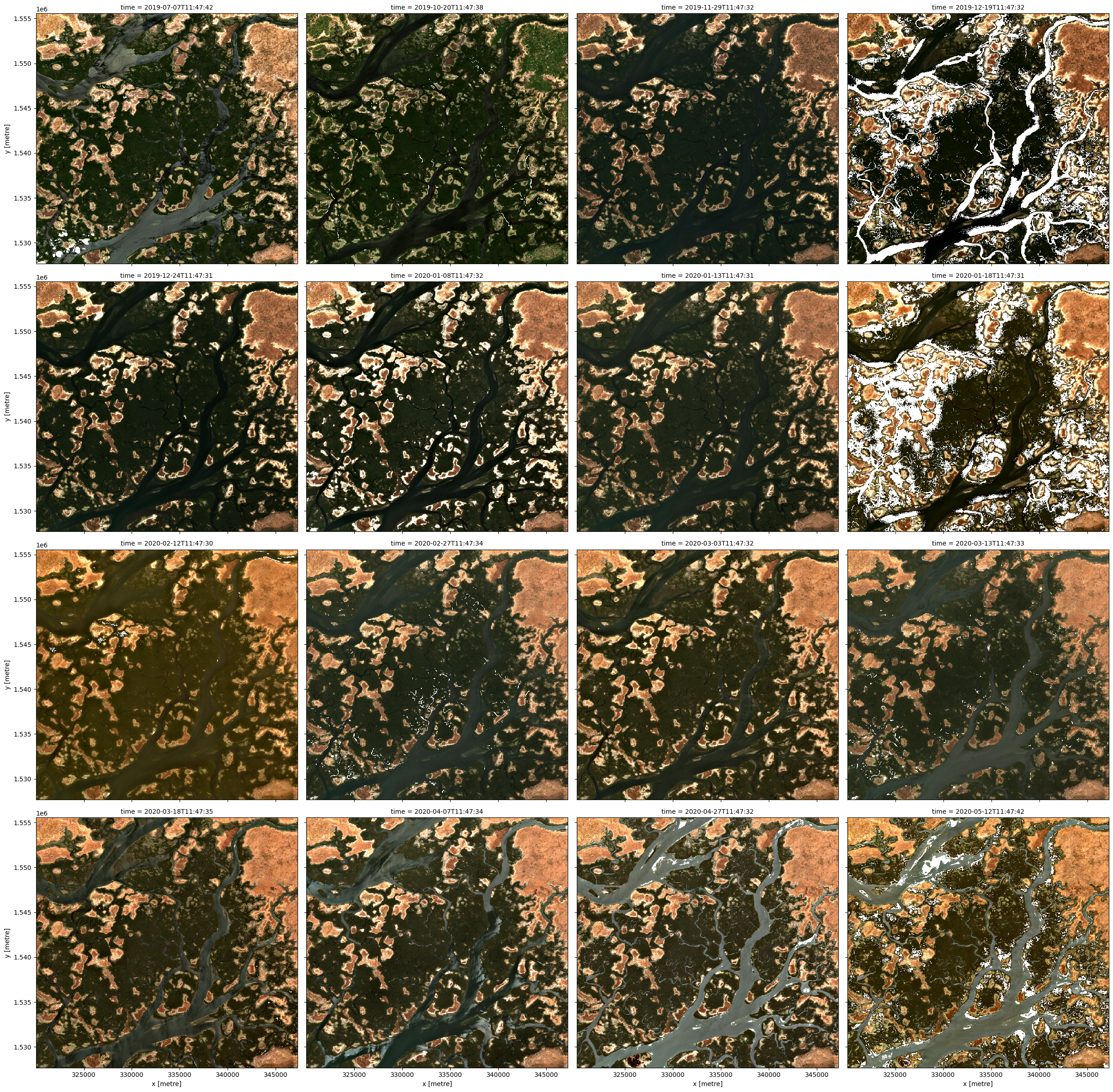
Tracez la première image pour voir à quoi ressemble notre zone

Nous pouvons utiliser la fonction « rgb » pour tracer les pas de temps dans notre ensemble de données sous forme d’images RVB en couleurs réelles :

[5]:

# Plot as an RGB image

rgb(ds, col='time')

../../../_images/sandbox_notebooks_Frequently_used_code_Calculating_band_indices_14_0.png

Calculer manuellement un indice

L’un des indices de télédétection les plus couramment utilisés est l’indice de végétation par différence normalisée ou « NDVI ». Cet indice utilise le rapport entre les bandes rouge et proche infrarouge (NIR) pour identifier la végétation verte vivante. La formule du NDVI est la suivante :

\[\begin{split}\begin{aligned} \text{NDVI} & = \frac{(\text{NIR} - \text{Rouge})}{(\text{NIR} + \text{Rouge})} \\ \end{aligned}\end{split}\]

Lors de l’interprétation de cet indice, les valeurs élevées indiquent la végétation et les valeurs faibles indiquent le sol ou l’eau.

[6]:

# Calculate NDVI using the formula above
ds['NDVI_manual'] = (ds.nir - ds.red) / (ds.nir + ds.red)

# Plot the results for one time step to see what they look like:
ds.NDVI_manual.plot(col='time', vmin=-0.50, vmax=0.8, cmap='RdYlGn')

[6]:

<xarray.plot.facetgrid.FacetGrid at 0x7f4d21379ac0>

../../../_images/sandbox_notebooks_Frequently_used_code_Calculating_band_indices_16_1.png

Dans l’image ci-dessus, la végétation apparaît en vert (NDVI > 0). Le sable apparaît en jaune (NDVI ~ 0) et l’eau apparaît en rouge (NDVI < 0).

Utilisez la fonction « calculate_indices » pour calculer un indice

La fonction « calculate_indices » fournit un moyen plus simple de calculer une large gamme d’indices de télédétection, notamment :

ASI (Indice de surface artificielle, Yongquan Zhao et Zhe Zhu 2022)
AWEI_ns (Indice d’extraction automatique de l’eau, sans ombres, Feyisa 2014)
AWEI_sh (Indice d’extraction automatique d’eau, ombres, Feyisa 2014)
BAEI (Indice d’extraction des zones bâties, Bouzekri et al. 2015)
BAI (Indice de surface brûlée, Martin 1998)
BSI (Indice de sol nu, Rikimaru et al. 2002)
BUI (Indice de constitution, He et al. 2010)
CMR (Rapport des minéraux argileux, Drury 1987)
ENDISI (Indice de différence normalisée améliorée pour les surfaces imperméables, Chen et al. 2019)
EVI (Indice de végétation amélioré, Huete 2002)
FMR (Ratio des minéraux ferreux, Segal 1982)
IOR (rapport d’oxyde de fer, Segal 1982)
LAI (indice de surface foliaire, Boegh 2002)
MBI (Indice de sol nu modifié, Nguyen et al. 2021)
MNDWI (Indice de différence normalisée de l’eau modifié, Xu 1996)
MSAVI (Indice de végétation ajusté au sol modifié, Qi et al. 1994)
NBI (Indice de construction neuve, Jieli et al. 2010)
NBR (rapport de combustion normalisé, Lopez Garcia 1991)
NDBI (Indice de différence normalisée, Zha 2003)
NDCI (Indice de différence normalisée de chlorophylle, Mishra & Mishra, 2012)
NDMI (Indice d’humidité par différence normalisée, Gao 1996)
NDSI (Indice de différence normalisée de neige, Hall 1995)
NDTI (Indice de turbidité par différence normalisée, Lacaux et al. 2007)
NDVI (Indice de végétation par différence normalisée, Rouse 1973)
NDWI (Indice de différence normalisée de l’eau, McFeeters 1996)
SAVI (Indice de végétation ajusté au sol, Huete 1988)
TCB (Brillance du bonnet à pompons, Crist 1985)
TCG (Casquette à pompons Greeness, Crist 1985)
TCW (humidité du bonnet à pompons, Crist 1985)
WI (Indice de l’eau, Fisher 2016)

La fonction calculate_indices se trouve dans le script deafrica_tools.bandindices. Ce script fournit toutes les opérations mathématiques nécessaires à la création de chaque index et mérite d’être examiné.

Utilisation de « calculate_indices » pour calculer plusieurs indices à la fois

La fonction « calculate_indices » permet de calculer facilement plusieurs indices de télédétection en une seule ligne de code.

Dans l’exemple ci-dessous, nous allons calculer le « NDVI » ainsi que deux indices d’eau courants : l’indice d’eau par différence normalisée (« NDWI ») et l’indice d’eau par différence normalisée modifiée (« MNDWI »). Les nouveaux indices apparaîtront dans la liste des « data_variables » ci-dessous :

[9]:

# Calculate multiple indices
ds_multi = calculate_indices(ds, index=['NDVI', 'NDWI', 'MNDWI'], satellite_mission='s2')

print(ds_multi)

<xarray.Dataset> Size: 594MB
Dimensions:      (time: 16, y: 929, x: 908)
Coordinates:
  * time         (time) datetime64[ns] 128B 2019-07-07T11:47:42 ... 2020-05-1...
  * y            (y) float64 7kB 1.556e+06 1.556e+06 ... 1.528e+06 1.528e+06
  * x            (x) float64 7kB 3.2e+05 3.201e+05 ... 3.472e+05 3.472e+05
    spatial_ref  int32 4B 32628
Data variables:
    red          (time, y, x) float32 54MB 2.965e+03 2.463e+03 ... nan nan
    green        (time, y, x) float32 54MB 2.132e+03 1.751e+03 ... nan nan
    blue         (time, y, x) float32 54MB 1.119e+03 921.0 1.285e+03 ... nan nan
    swir_1       (time, y, x) float32 54MB 5.63e+03 5.547e+03 ... nan nan
    swir_2       (time, y, x) float32 54MB 5.131e+03 4.916e+03 ... nan nan
    nir          (time, y, x) float32 54MB 4.045e+03 3.745e+03 ... nan nan
    nir_2        (time, y, x) float32 54MB 4.177e+03 4.228e+03 ... nan nan
    NDVI_manual  (time, y, x) float32 54MB 0.1541 0.2065 0.1487 ... nan nan nan
    NDVI         (time, y, x) float32 54MB 0.1541 0.2065 0.1487 ... nan nan nan
    NDWI         (time, y, x) float32 54MB -0.3097 -0.3628 -0.2971 ... nan nan
    MNDWI        (time, y, x) float32 54MB -0.4507 -0.5201 -0.4452 ... nan nan
Attributes:
    crs:           EPSG:32628
    grid_mapping:  spatial_ref

[10]:

# Plot the NDWI results
ds_multi.NDWI.plot(col='time', robust=True, cmap='PuBu')

[10]:

<xarray.plot.facetgrid.FacetGrid at 0x7f4d212ab380>

../../../_images/sandbox_notebooks_Frequently_used_code_Calculating_band_indices_25_1.png

[11]:

# Plot the MNDWI results
ds_multi.MNDWI.plot(col='time', robust=True, cmap='PuBu')

[11]:

<xarray.plot.facetgrid.FacetGrid at 0x7f4d200a35c0>

../../../_images/sandbox_notebooks_Frequently_used_code_Calculating_band_indices_26_1.png

Nous pouvons également supprimer les bandes satellites d’origine de l’ensemble de données à l’aide de « drop=True ». L’ensemble de données produit ci-dessous ne doit désormais inclure que les nouvelles bandes « NDVI », « NDWI », « MNDWI » sous « data_variables » :

[12]:

# Calculate multiple indices and drop original bands
ds_drop = calculate_indices(ds, index=['NDVI', 'NDWI', 'MNDWI'], drop=True, satellite_mission='s2')
print(ds_drop)

Dropping bands ['red', 'green', 'blue', 'swir_1', 'swir_2', 'nir', 'nir_2', 'NDVI_manual']
<xarray.Dataset> Size: 162MB
Dimensions:      (time: 16, y: 929, x: 908)
Coordinates:
  * time         (time) datetime64[ns] 128B 2019-07-07T11:47:42 ... 2020-05-1...
  * y            (y) float64 7kB 1.556e+06 1.556e+06 ... 1.528e+06 1.528e+06
  * x            (x) float64 7kB 3.2e+05 3.201e+05 ... 3.472e+05 3.472e+05
    spatial_ref  int32 4B 32628
Data variables:
    NDVI         (time, y, x) float32 54MB 0.1541 0.2065 0.1487 ... nan nan nan
    NDWI         (time, y, x) float32 54MB -0.3097 -0.3628 -0.2971 ... nan nan
    MNDWI        (time, y, x) float32 54MB -0.4507 -0.5201 -0.4452 ... nan nan
Attributes:
    crs:           EPSG:32628
    grid_mapping:  spatial_ref

Informations Complémentaires

Licence : Le code de ce carnet est sous licence Apache, version 2.0 <https://www.apache.org/licenses/LICENSE-2.0>. Les données de Digital Earth Africa sont sous licence Creative Commons par attribution 4.0 <https://creativecommons.org/licenses/by/4.0/>.

Contact : Si vous avez besoin d’aide, veuillez poster une question sur le canal Slack Open Data Cube <http://slack.opendatacube.org/>`__ ou sur le GIS Stack Exchange en utilisant la balise open-data-cube (vous pouvez consulter les questions posées précédemment ici). Si vous souhaitez signaler un problème avec ce bloc-notes, vous pouvez en déposer un sur Github.

Version de Datacube compatible :

[13]:

print(datacube.__version__)

1.9.13

Dernier test :

[14]:

from datetime import date
print(date.today())

2026-04-08