Water detection with Sentinel-1

• Produits utilisés : s1_rtc

Mots-clés : données utilisées ; sentinel-1,:index:SAR, eau

Aperçu

Plus de 40 % de la population mondiale vit à moins de 100 km du littoral. Cependant, les environnements côtiers sont en constante évolution, l’érosion et les changements côtiers représentant un défi majeur pour les infrastructures côtières précieuses et les habitats écologiques importants. La mise à jour des données sur la position du littoral est essentielle pour que les gestionnaires côtiers puissent identifier et minimiser les impacts des changements côtiers et de l’érosion. Les régions côtières abritent également de nombreuses zones humides. La surveillance de l’étendue des eaux aide à comprendre et à protéger ces écosystèmes dynamiques et productifs.

Bien que les côtes et les étendues d’eau puissent être cartographiées à l’aide de données optiques (comme le montre le Coastal Erosion notebook), ces images peuvent être fortement affectées par la météo, notamment par la présence de nuages, qui obscurcissent la terre et l’eau en dessous. Cela peut être un problème particulier dans les régions nuageuses ou dans les zones où les nuages pendant la saison des pluies empêchent les satellites optiques de prendre des images claires pendant de nombreux mois de l’année.

Les observations radar ne sont pas affectées par la couverture nuageuse. Les deux satellites Sentinel-1, exploités par l’ESA dans le cadre du programme Copernicus, fournissent des observations par tous les temps tous les 6 à 12 jours au-dessus de l’Afrique. En développant un processus de classification des pixels observés en eau ou en terre, il est possible d’identifier le littoral et de cartographier les étendues d’eau dynamiques à l’aide de données radar. Pour plus d’informations, consultez le bloc-notes Sentinel-1.

Description

Dans cet exemple, nous utilisons les données des satellites Sentinel-1 pour créer un classificateur capable de déterminer si un pixel est une étendue d’eau ou une étendue d’eau. Plus précisément, ce bloc-notes utilise la rétrodiffusion radar prête à l’emploi, qui décrit la force du signal reçu par le satellite.

Le cahier contient les étapes suivantes :

1. Chargez les données de rétrodiffusion Sentinel-1 pour une zone d’intérêt et visualisez les données renvoyées

2. Application d’un filtre speckle et conversion des nombres numériques en valeurs dB pour l’analyse

3. Utiliser l’analyse d’histogramme pour déterminer le seuil de classification de l’eau

4. Concevoir un classificateur pour distinguer la terre et l’eau

5. Appliquer le classificateur à la zone d’intérêt et interpréter les résultats

---

Commencer

Pour exécuter cette analyse, exécutez toutes les cellules du bloc-notes, en commençant par la cellule « Charger les packages ».

Charger des paquets

Importez les packages Python utilisés pour l’analyse.

%matplotlib inline

import os
import warnings
import datacube
import numpy as np
import xarray as xr
import geopandas as gpd
import matplotlib.pyplot as plt
warnings.filterwarnings("ignore")

from scipy.ndimage.filters import uniform_filter
from scipy.ndimage.measurements import variance
from skimage.filters import threshold_minimum
from odc.geo.geom import Geometry
from deafrica_tools.spatial import xr_rasterize
from deafrica_tools.datahandling import load_ard
from deafrica_tools.plotting import display_map, rgb
from deafrica_tools.areaofinterest import define_area

Se connecter au datacube

Connectez-vous au datacube pour que nous puissions accéder aux données DEA. Le paramètre « app » est un nom unique pour l’analyse qui est basé sur le nom du fichier du notebook.

dc = datacube.Datacube(app="Radar_water_detection")

Paramètres d’analyse

La cellule suivante définit les paramètres qui définissent la zone d’intérêt et la durée de l’analyse. Les paramètres sont

• « lat » : la latitude centrale à analyser (par exemple « 10,338 »).

• « lon » : la longitude centrale à analyser (par exemple « -1,055 »).

• « buffer » : le nombre de degrés carrés à charger autour de la latitude et de la longitude centrales. Pour des temps de chargement raisonnables, définissez cette valeur sur « 0,1 » ou moins.

• time_range : la plage de dates à analyser (par exemple, ('2020'))

Si vous exécutez le bloc-notes pour la première fois, conservez les paramètres par défaut ci-dessous. Cela montrera comment fonctionne l’analyse et fournira des résultats significatifs. L’exemple couvre la côte de Ziguinchor, en Gambie.

Sélectionnez l’emplacement

Pour définir la zone d’intérêt, deux méthodes sont disponibles :

1. En spécifiant la latitude, la longitude et la zone tampon. Cette méthode nécessite que vous saisissiez la latitude centrale, la longitude centrale et la valeur de la zone tampon en degrés carrés autour du point central que vous souhaitez analyser. Par exemple, « lat = 10,338 », « lon = -1,055 » et « buffer = 0,1 » sélectionneront une zone avec un rayon de 0,1 degré carré autour du point avec les coordonnées (10,338, -1,055).

   Vous pouvez également fournir des valeurs de tampon distinctes pour la latitude et la longitude d’une zone rectangulaire. Par exemple, « lat = 10.338 », « lon = -1.055 » et « lat_buffer = 0.1 » et « lon_buffer = 0.08 » sélectionneront une zone rectangulaire s’étendant sur 0,1 degré au nord et au sud et 0,08 degré à l’est et à l’ouest à partir du point « (10.338, -1.055) ».

   Pour des temps de chargement raisonnables, définissez la mémoire tampon sur « 0,1 » ou moins.

2. By uploading a polygon as a GeoJSON or Esri Shapefile. If you choose this option, you will need to upload the geojson or ESRI shapefile into the Sandbox using Upload Files button in the top left corner of the Jupyter Notebook interface. ESRI shapefiles must be uploaded with all the related files (.cpg, .dbf, .shp, .shx). Once uploaded, you can use the shapefile or geojson to define the area of interest. Remember to update the code to call the file you have uploaded.

Pour utiliser l’une de ces méthodes, vous pouvez décommenter la ligne de code concernée et commenter l’autre. Pour commenter une ligne, ajoutez le symbole "#" avant le code que vous souhaitez commenter. Par défaut, la première option qui définit l’emplacement à l’aide de la latitude, de la longitude et du tampon est utilisée.

La latitude et la longitude sélectionnées seront affichées sous forme de cadre rouge sur la carte sous la cellule suivante. Cette carte peut être utilisée pour trouver les coordonnées d’autres lieux. Faites simplement défiler la carte et cliquez sur n’importe quel point pour afficher la latitude et la longitude de cet endroit.

# Method 1: Specify the latitude, longitude, and buffer
aoi = define_area(lat=12.62, lon=-16.29, buffer=0.05)

# Method 2: Use a polygon as a GeoJSON or Esri Shapefile.
#aoi = define_area(vector_path='aoi.shp')

#Create a geopolygon and geodataframe of the area of interest
geopolygon = Geometry(aoi["features"][0]["geometry"], crs="epsg:4326")
geopolygon_gdf = gpd.GeoDataFrame(geometry=[geopolygon], crs=geopolygon.crs)

# Get the latitude and longitude range of the geopolygon
lat_range = (geopolygon_gdf.total_bounds[1], geopolygon_gdf.total_bounds[3])
lon_range = (geopolygon_gdf.total_bounds[0], geopolygon_gdf.total_bounds[2])

#timeframe
timerange = ('2020')

Afficher l’emplacement sélectionné

La cellule suivante affichera la zone sélectionnée sur une carte interactive. N’hésitez pas à zoomer et dézoomer pour mieux comprendre la zone que vous allez analyser. En cliquant sur n’importe quel point de la carte, vous découvrirez les coordonnées de latitude et de longitude de ce point.

display_map(x=lon_range, y=lat_range)

Make this Notebook Trusted to load map: File -> Trust Notebook

Charger et afficher les données Sentinel-1

La première étape de l’analyse consiste à charger les données de rétrodiffusion Sentinel-1 pour la zone d’intérêt spécifiée. Cela utilise la fonction utilitaire prédéfinie load_ard.

Veuillez être patient. Le chargement des données peut prendre quelques minutes et la progression sera indiquée par une sortie texte. Le chargement est terminé lorsque l’état de la cellule passe de « [*] » à « [numéro] ».

# Load the Sentinel-1 data
S1 = load_ard(dc=dc,
              products=["s1_rtc"],
              measurements=['vv', 'vh'],
              y=lat_range,
              x=lon_range,
              time=timerange,
              output_crs = "EPSG:6933",
              resolution = (-20,20),
              group_by="solar_day",
              dtype='native'
             )

Using pixel quality parameters for Sentinel 1
Finding datasets
    s1_rtc
Applying pixel quality/cloud mask
Loading 31 time steps

Une fois le chargement terminé, examinez les données en les imprimant dans la cellule suivante. L’argument « Dimensions » révèle le nombre d’intervalles de temps dans l’ensemble de données, ainsi que le nombre de pixels dans les dimensions « x » (longitude) et « y » (latitude).

print(S1)

<xarray.Dataset> Size: 75MB
Dimensions:      (time: 31, y: 623, x: 484)
Coordinates:
  * time         (time) datetime64[ns] 248B 2020-01-04T19:17:46.582116 ... 20...
  * y            (y) float64 5kB 1.604e+06 1.604e+06 ... 1.591e+06 1.591e+06
  * x            (x) float64 4kB -1.577e+06 -1.577e+06 ... -1.567e+06 -1.567e+06
    spatial_ref  int32 4B 6933
Data variables:
    vv           (time, y, x) float32 37MB 0.05976 0.04359 ... 0.1871 0.1521
    vh           (time, y, x) float32 37MB 0.005369 0.004237 ... 0.01575 0.01733
Attributes:
    crs:           EPSG:6933
    grid_mapping:  spatial_ref

Visualiser la série chronologique

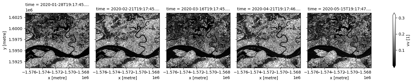
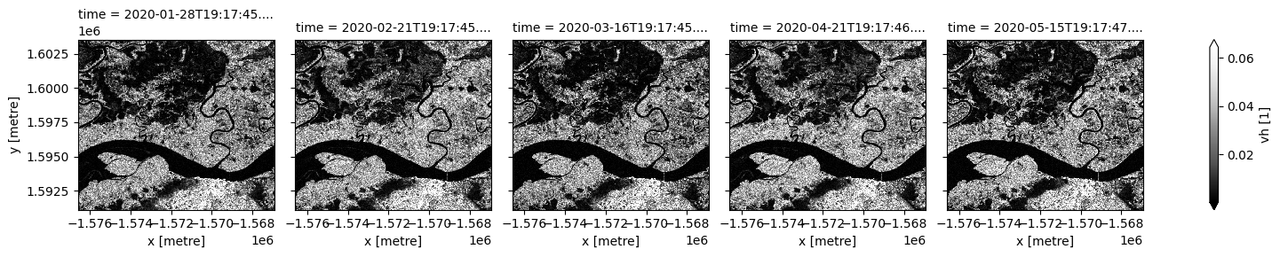
Les zones côtières et humides sont très dynamiques, c’est pourquoi une évaluation sans nuages à l’aide d’un radar est utile pour capturer les changements en toutes saisons. Dans les cellules suivantes, les observations de Sentinel-1 dans différentes polarisations sont représentées pour des dates sélectionnées. Notons que la rétrodiffusion VV est généralement significativement plus élevée que VH. Les signaux des deux polarisations sont dominés par des mécanismes de diffusion différents et réagissent donc différemment aux caractéristiques de surface.

Les deux polarisations montrent un changement significatif de la couverture de surface au fil du temps. L’eau libre est caractérisée par une faible rétrodiffusion due à la réflexion spéculaire. La zone d’eau avec végétation debout entraîne une rétrodiffusion élevée et ne sera pas cartographiée à l’aide de la méthode de seuillage ci-dessous. Cela peut entraîner une mesure de l’étendue d’eau différente par rapport aux méthodes utilisant des données optiques.

#Selecting a few images from the loaded S1 to visualise
timesteps = [2,4,6,9,11]

# Plot VV polarisation for specific timeframe
S1.vv.isel(time=timesteps).plot(cmap="Greys_r", robust=True, col="time", col_wrap=5);

# Plot VH polarisation for specific timeframe
S1.vh.isel(time=timesteps).plot(cmap="Greys_r", robust=True, col="time", col_wrap=5);

Les mesures de rétrodiffusion peuvent être combinées dans la visualisation pour mettre en évidence les différentes signatures de polarisation. Pour la visualisation RVB ci-dessous, le rapport entre VH et VV est ajouté comme troisième bande de mesure.

# VH/VV is a potentially useful third feature after VV and VH
S1['vh/vv'] = S1.vh/S1.vv

# median values are used to scale the measurements so they have a similar range for visualization
med_s1 = S1[['vv','vh','vh/vv']].median()

# plotting an RGB image for selected timesteps
rgb(S1[['vv', 'vh', 'vh/vv']]/med_s1, bands=['vv',
    'vh', 'vh/vv'], index=timesteps, col_wrap=5);

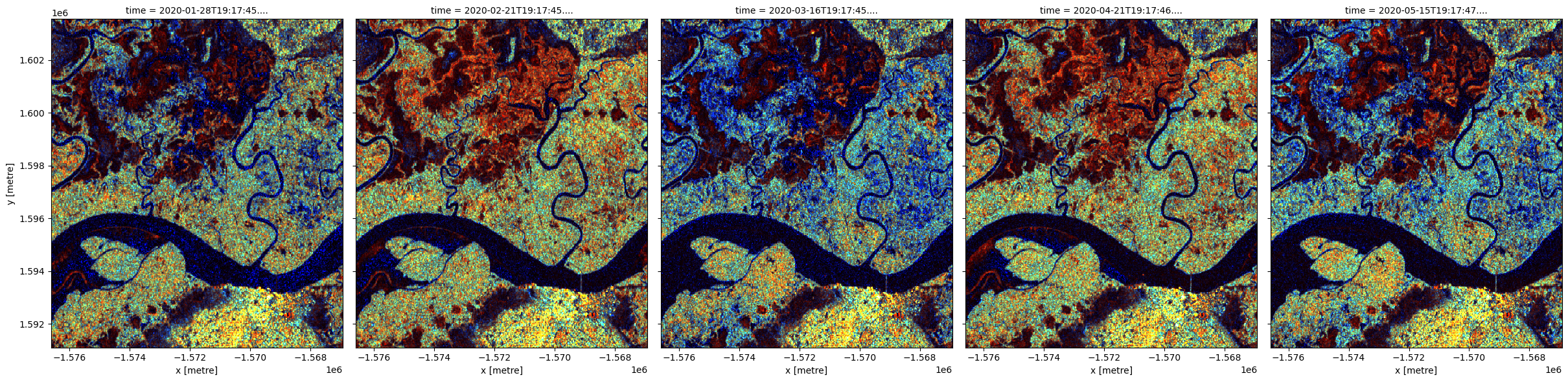
Des changements significatifs dans le schéma de couleur sont visibles d’un mois à l’autre. Les eaux libres et les surfaces lisses et nues apparaissent en bleu foncé car toutes les mesures sont faibles. La couverture arborée apparaît en cyan en raison du signal VH relativement plus élevé dû à la diffusion du volume. Les zones en rouge vif sont probablement des eaux avec de la végétation debout. La zone urbaine est indiquée en jaune vif au bas des images.

Appliquer le filtrage des taches

Les observations radar apparaissent mouchetées en raison de l’interférence aléatoire de signaux cohérents provenant de la diffusion de la cible. Le bruit moucheté peut être réduit en faisant la moyenne des valeurs de pixels sur une zone ou dans le temps. Cependant, le calcul de la moyenne sur une fenêtre fixe atténue les variations spatiales locales réelles et conduit à une résolution spatiale réduite. Une approche adaptative qui prend en compte l’homogénéité locale est donc préférable.

Ci-dessous, nous appliquons le filtre Lee, l’un des filtres speckle adaptatifs les plus populaires.

#defining a function to apply lee filtering on S1 image
def lee_filter(da, size):
    """
    Apply lee filter of specified window size.
    Adapted from https://stackoverflow.com/questions/39785970/speckle-lee-filter-in-python

    """
    img = da.values
    img_mean = uniform_filter(img, size)
    img_sqr_mean = uniform_filter(img**2, size)
    img_variance = img_sqr_mean - img_mean**2

    overall_variance = variance(img)

    img_weights = img_variance / (img_variance + overall_variance)
    img_output = img_mean + img_weights * (img - img_mean)

    return img_output

Maintenant que nous avons défini le filtre, nous pouvons l’exécuter sur les données VV et VH. Vous avez peut-être remarqué que la fonction prend un argument de taille. Cela modifiera le degré de flou de l’image après le lissage. Nous avons choisi une valeur par défaut pour cette analyse, mais vous pouvez l’expérimenter si cela vous intéresse.

# The lee filter above doesn't handle null values
# We therefore set null values to 0 before applying the filter
valid = np.isfinite(S1)
S1 = S1.where(valid, 0)

# Create a new entry in dataset corresponding to filtered VV and VH data
S1["filtered_vv"] = S1.vv.groupby("time").apply(lee_filter, size=7)
S1["filtered_vh"] = S1.vh.groupby("time").apply(lee_filter, size=7)

# Null pixels should remain null
S1['filtered_vv'] = S1.filtered_vv.where(valid.vv)
S1['filtered_vh'] = S1.filtered_vh.where(valid.vh)

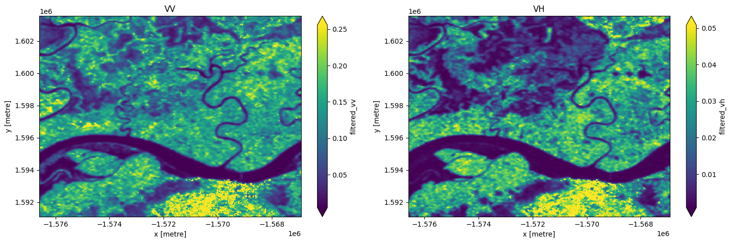
# images appear smoother after speckle filtering
fig, ax = plt.subplots(1, 2, figsize=(15,5))
S1["filtered_vv"].isel(time=3).plot(ax = ax[0],robust=True)
S1["filtered_vh"].isel(time=3).plot(ax = ax[1],robust=True);
ax[0].set_title('VV')
ax[1].set_title('VH')
plt.tight_layout();

Convertir les nombres numériques en dB

Bien que la rétrodiffusion Sentinel-1 soit fournie sous forme d’intensité linéaire, il est souvent utile de convertir la rétrodiffusion en décibels (dB) pour l’analyse. La rétrodiffusion en dB présente un profil de bruit plus symétrique et une distribution de valeurs moins biaisée pour une évaluation statistique plus facile.

S1['filtered_vv'] = 10 * np.log10(S1.filtered_vv)
S1['filtered_vh'] = 10 * np.log10(S1.filtered_vh)

Analyse d’histogramme pour Sentinel-1

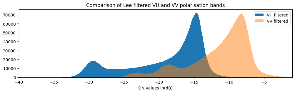
Les distributions de rétrodiffusion sont représentées ci-dessous sous forme d’histogrammes.

fig = plt.figure(figsize=(12, 3))
S1.filtered_vh.plot.hist(bins=1000, label="VH filtered")
S1.filtered_vv.plot.hist(bins=1000, label="VV filtered",alpha=0.5)
plt.xlim(-40,-1)
plt.legend()
plt.xlabel("DN values in(dB)")
plt.title("Comparison of Lee filtered VH and VV polarisation bands");

Construire et appliquer le classificateur

L’histogramme de rétrodiffusion VH montre une distribution bimodale avec des valeurs faibles sur l’eau et des valeurs élevées sur la terre. L’histogramme VV présente plusieurs pics et une séparation moins évidente entre l’eau et la terre.

Nous construisons donc un classifieur basé sur la rétrodiffusion VH. Nous choisissons un seuil pour séparer la terre et l’eau : les pixels avec des valeurs inférieures au seuil sont de l’eau, et les pixels avec des valeurs supérieures au seuil ne sont pas de l’eau (terre).

Il existe plusieurs façons de déterminer le seuil. Ici, nous utilisons la fonction « threshod_minimum » implémentée dans le package « skimage » pour déterminer automatiquement le seuil à partir de l’histogramme VH. Cette méthode calcule l’histogramme pour toutes les valeurs de rétrodiffusion, le lisse jusqu’à ce qu’il n’y ait que deux maxima et trouve le minimum entre les deux comme seuil.

threshold_vh = threshold_minimum(S1.filtered_vh.values)

print(threshold_vh)

-25.55214938754847

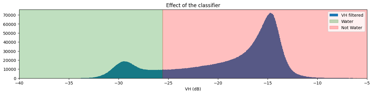
Visualiser le seuil

Pour vérifier si notre seuil choisi divise raisonnablement les deux distributions, nous pouvons ajouter le seuil aux tracés d’histogramme que nous avons réalisés précédemment.

fig, ax = plt.subplots(figsize=(15, 3))
S1.filtered_vh.plot.hist(bins=1000, label="VH filtered")
plt.xlim(-40,-5)
ax.axvspan(xmin=-40.0, xmax=threshold_vh, alpha=0.25, color="green", label="Water")
ax.axvspan(xmin=threshold_vh,
           xmax=-5,
           alpha=0.25,
           color="red",
           label="Not Water")
plt.legend()
plt.xlabel("VH (dB)")
plt.title("Effect of the classifier")
plt.show()

Définir le classificateur

Ce seuil est utilisé pour écrire une fonction qui renvoie uniquement les pixels classés comme eau. Les étapes de base que la fonction exécutera sont les suivantes :

1. Rechercher tous les pixels qui ont des valeurs filtrées inférieures au seuil ; ce sont les pixels « eau ».

2. Renvoie un ensemble de données contenant les pixels « eau ».

def S1_water_classifier(da, threshold=threshold_vh):
    water_data_array = da < threshold
    return water_data_array.to_dataset(name="s1_water")

Maintenant que nous avons défini la fonction de classification, nous pouvons l’appliquer aux données. Après avoir exécuté le classificateur, nous pourrons visualiser le produit de données classifié en exécutant « print(S1.water) ».

S1['water'] = S1_water_classifier(S1.filtered_vh).s1_water

Évaluation avec la moyenne

Nous pouvons maintenant visualiser l’image avec notre classification. Le classificateur renvoie soit « True » soit « False » pour chaque pixel. Pour détecter les limites des éléments aquatiques, nous voulons vérifier quels pixels sont toujours de l’eau et lesquels sont toujours de la terre. De manière pratique, Python encode « True = 1 » et « False = 0 ».

Si nous traçons la valeur moyenne des pixels classés, les pixels qui sont toujours de l’eau auront une valeur moyenne de « 1 » et les pixels qui sont toujours de la terre auront une moyenne de « 0 ». Les pixels qui sont parfois de l’eau et parfois de la terre auront une moyenne entre ces valeurs. Dans cette étude de cas, ces pixels sont associés à des zones humides inondées de façon saisonnière.

La cellule suivante trace la valeur moyenne des pixels classés, ou la fréquence de détection de l’eau, au fil du temps.

# Plot the mean of each classified pixel value
plt.figure(figsize=(8, 7))
S1.water.mean(dim='time').plot(cmap="RdBu")
plt.title("Average classified pixel value");

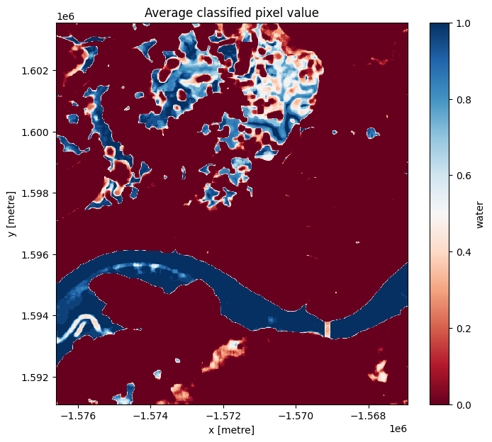
Vous pouvez voir que le seuil sélectionné a fait du bon travail en séparant les pixels d’eau (en bleu) et les pixels terrestres (en rouge) ainsi que les éléments d’eau éphémères entre les deux.

Vous devriez pouvoir voir que le littoral prend un mélange de valeurs entre « 0 » et « 1 », mettant en évidence des pixels qui sont parfois terrestres et parfois aquatiques. Cela est probablement dû à l’effet des marées montantes et descendantes, certaines observations radar étant capturées à marée basse et d’autres à marée haute.

Évaluation avec écart type

Étant donné que nous avons identifié le rivage comme les pixels qui sont classés parfois comme terre et parfois comme eau, nous pouvons également voir si l’écart type de chaque pixel au fil du temps est un moyen raisonnable de déterminer si un pixel est un rivage ou non.

De la même manière que nous avons calculé et tracé la moyenne ci-dessus, vous pouvez calculer et tracer l’écart type en utilisant la fonction « std » à la place de la fonction « mean ».

Si vous souhaitez voir les résultats en utilisant une palette de couleurs différente, vous pouvez également essayer de remplacer « cmap= »Greys »`` ou « cmap= »Blues »`` par « cmap= »viridis »`` ».

plt.figure(figsize=(8, 7))
S1.water.std(dim="time").plot(cmap="viridis")
plt.title("Standard deviation of classified pixel values");

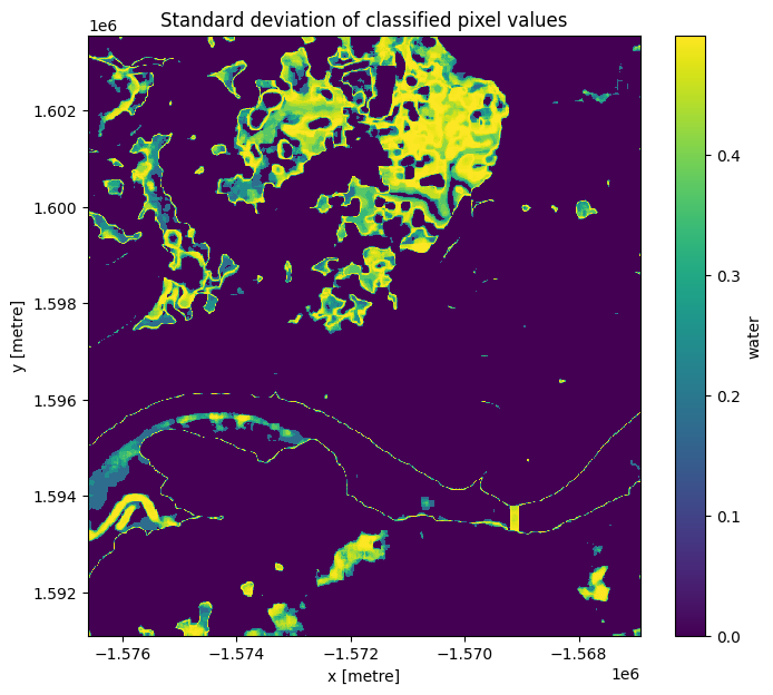
L’écart type que nous avons calculé ci-dessus nous donne une idée de la variabilité d’un pixel sur toute la période de temps que nous avons examinée. À partir de l’image ci-dessus, vous devriez pouvoir voir que les pixels terrestres et aquatiques ont presque toujours un écart type de « 0 », ce qui signifie qu’ils n’ont pas changé au cours de la période où nous avons échantillonné. Le littoral et les zones humides ont cependant un écart type plus élevé, ce qui indique qu’ils changent fréquemment entre l’eau et le non-eau.

Il est important de reconnaître que l’écart type peut ne pas être en mesure de détecter la différence entre le bruit, les marées et le changement en cours, car un pixel qui alterne fréquemment entre la terre et l’eau (bruit) pourrait avoir le même écart type qu’un pixel qui est terre pendant un certain temps, puis devient eau pendant le temps restant (changement en cours ou marées).

Prochaines étapes

Une fois terminé, revenez à la section « Paramètres d’analyse », modifiez certaines valeurs (par exemple lat et lon) et relancez l’analyse. Vous pouvez utiliser la carte interactive dans la section « Afficher l’emplacement sélectionné » pour trouver de nouvelles valeurs de latitude et de longitude centrales en effectuant un panoramique et un zoom, puis en cliquant sur la zone pour laquelle vous souhaitez extraire les valeurs de localisation. Vous pouvez également utiliser Google Maps pour rechercher un emplacement que vous connaissez, puis renvoyer les valeurs de latitude et de longitude en cliquant sur la carte.

---

Informations Complémentaires

Licence Le code de ce notebook est sous licence Apache, version 2.0 <https://www.apache.org/licenses/LICENSE-2.0>`__.

Les données de Digital Earth Africa sont sous licence Creative Commons Attribution 4.0 <https://creativecommons.org/licenses/by/4.0/>.

Contact Si vous avez besoin d’aide, veuillez poster une question sur le canal Slack DE Africa <https://digitalearthafrica.slack.com/> ou sur le GIS Stack Exchange <https://gis.stackexchange.com/questions/ask?tags=open-data-cube> en utilisant la balise open-data-cube (vous pouvez consulter les questions posées précédemment `ici <https://gis.stackexchange.com/questions/tagged/open-data-

Si vous souhaitez signaler un problème avec ce notebook, vous pouvez en déposer un sur Github.

Version de Datacube compatible

print(datacube.__version__)

1.8.20

Dernier test :

from datetime import datetime
datetime.today().strftime('%Y-%m-%d')

'2025-12-11'