Anomalies mensuelles de l’état de la végétation
Products used: ndvi_climatology_ls, crop_mask, wofs_ls_summary_alltime, s2_l2a_c1, ls8_sr, ls9_sr
Mots clés: données utilisées; ndvi_climatology_ls, végétation; anomalies, indice de bande; NDVI;
Aperçu
Pour comprendre comment le paysage végétal réagit aux facteurs environnementaux à long terme tels que l’oscillation australe El Niño (ENSO) ou le changement climatique, il faut calculer des anomalies standardisées. Les anomalies standardisées soustraient la moyenne à long terme d’une observation d’intérêt, puis divisent le résultat par l’écart type à long terme, supprimant ainsi la variabilité saisonnière et mettant en évidence les changements liés aux facteurs à long terme.
Description
This notebook will calculate monthly standardised NDVI anomalies for any given month and year, and relies on DE Africa’s 30 metre resolution NDVI climatology product to define the baseline vegetation condition. Sentinel-2 c1, and Landsat 8/9 are used to calculate the monthly mean NDVI for the month of interest. The standardised anaomaly is then calculated as:
\begin{equation} \text{Anomalie normalisée}=\frac{x-m}{s} \end{equation}
où \(x\) est le NDVI pour le mois d’intérêt, \(m\) est la moyenne à long terme et \(s\) est l’écart type à long terme.
Les étapes suivantes sont décrites dans le notebook :
Charger un polygone pour le pays d’intérêt (un geojson avec les frontières des pays est déjà fourni)
Load cloud masked Sentinel-2 c1 and Landsat satellite data
Prétraiter les données satellite afin d’obtenir une série chronologique continue et sans bruit de NDVI.
Créer un masque de frontière de pays
Charger le produit climatologique NDVI de DE Africa
Utilisez WOfS pour supprimer les plans d’eau de la région
Calculer les anomalies NDVI standardisées
Tracer le résultat
Charger le masque de culture de DE Africa pour la région
Tracer les anomalies NDVI pour les régions uniquement dans le masque de culture
Commencer
Pour exécuter cette analyse, exécutez toutes les cellules du bloc-notes, en commençant par la cellule « Charger les packages ».
Une fois l’analyse terminée, revenez à la cellule « Paramètres d’analyse », modifiez certaines valeurs (par exemple, choisissez un autre emplacement ou une autre période à analyser) et relancez l’analyse.
Charger des paquets
Chargez les principaux packages Python et les fonctions de support pour l’analyse.
[1]:
%matplotlib inline
import warnings
warnings.filterwarnings("ignore", category=FutureWarning)

import datacube
import xarray as xr
import numpy as np
import geopandas as gpd
import matplotlib.pyplot as plt
from datacube.utils import masking
from odc.geo.geom import Geometry
from odc.geo.crs import CRS
from deafrica_tools.spatial import xr_rasterize

from deafrica_tools.datahandling import load_ard
from deafrica_tools.bandindices import calculate_indices
from deafrica_tools.plotting import display_map
from deafrica_tools.dask import create_local_dask_cluster

import warnings
# Force ignore ALL future warnings at a deeper level
warnings.simplefilter("ignore", FutureWarning)
Configurer un cluster Dask
Dask peut être utilisé pour mieux gérer l’utilisation de la mémoire et effectuer l’analyse en parallèle. Pour une introduction à l’utilisation de Dask avec Digital Earth Africa, consultez le Dask notebook.
Remarque : nous vous recommandons d’ouvrir la fenêtre de traitement Dask pour afficher les différents calculs en cours d’exécution ; pour ce faire, consultez la section Tableau de bord Dask en Afrique de l’Ouest du Dask notebook.
Pour utiliser Dask, configurez le cluster de calcul local à l’aide de la cellule ci-dessous.
[2]:
create_local_dask_cluster()
/opt/venv/lib/python3.12/site-packages/distributed/node.py:188: UserWarning: Port 8787 is already in use.
Perhaps you already have a cluster running?
Hosting the HTTP server on port 33839 instead
  warnings.warn(
Client
Client-763fdddb-3752-11f1-91c4-66901f7a1b9b
| Connection method: Cluster object | Cluster type: distributed.LocalCluster |
| Dashboard: /user/mpho.sadiki@digitalearthafrica.org/proxy/33839/status |
Cluster Info
LocalCluster
51f936a1
| Dashboard: /user/mpho.sadiki@digitalearthafrica.org/proxy/33839/status | Workers: 1 |
| Total threads: 4 | Total memory: 26.21 GiB |
| Status: running | Using processes: True |
Scheduler Info
Scheduler
Scheduler-f36b4014-12cc-43c6-9287-335057ac42be
| Comm: tcp://127.0.0.1:42211 | Workers: 0 |
| Dashboard: /user/mpho.sadiki@digitalearthafrica.org/proxy/33839/status | Total threads: 0 |
| Started: Just now | Total memory: 0 B |
Workers
Worker: 0
| Comm: tcp://127.0.0.1:36927 | Total threads: 4 |
| Dashboard: /user/mpho.sadiki@digitalearthafrica.org/proxy/41845/status | Memory: 26.21 GiB |
| Nanny: tcp://127.0.0.1:42045 | |
| Local directory: /tmp/dask-scratch-space/worker-wi322xoz | |
Se connecter au datacube
Activez la base de données Datacube, qui fournit des fonctionnalités pour le chargement et l’affichage des données d’observation de la Terre stockées.
[3]:
dc = datacube.Datacube(app="Vegetation_anomalies")
Paramètres d’analyse
La cellule suivante définit des paramètres importants pour l’analyse :
« pays » : le pays sur lequel charger les données, par exemple « Ouganda ». La liste complète des pays africains se trouve dans la cellule « [6] »
« année » : l’année pour laquelle nous allons calculer l’anomalie standardisée, par exemple « 2022 »
« mois » : le mois pour lequel nous allons calculer l’anomalie standardisée, écrit sous la forme d’une abréviation de trois lettres minuscules, par exemple « jan », « fev », etc. Ceci est dû au fait que les mesures du produit « ndvi_climatology_ls » sont stockées sous la forme « mean_jan », « mean_feb », etc.
crop_mask: selon l’endroit où vous chargez les données, vous pouvez modifier le masque de recadrage à charger avec ce paramètre. Utilisez l’explorateur <https://explorer.digitalearth.africa/products>`__ pour trouver quel masque de recadrage couvre quelle région de l’Afrique.résolution: la résolution des cellules x et y des données satellite et des donnéesndvi_climatology_ls, par exemple(-30, 30)chargera les données à leur résolution native de 30 x 30 m. Si vous chargez une grande zone, augmentez la résolution pour que les données tiennent dans la mémoire. Par exemple, si vous essayez de trouver l’anomalie NDVI pour un grand pays, envisagez d’augmenter la résolution à(-210,210).dask_chunks: la taille des morceaux dask, dask divise les données en morceaux gérables qui peuvent être facilement stockés en mémoire, par exempledict(x=1000,y=1000)
Si vous exécutez le bloc-notes pour la première fois, conservez les paramètres par défaut ci-dessous. Cela permettra de démontrer le fonctionnement de l’analyse et de fournir des résultats significatifs.
[4]:
# Select a country
country = "Uganda"

# year and month for anomaly
year = "2023"
month = "jan"

# the crop mask to use
crop_mask = "crop_mask"

# pixel resolution can got as low as (-30,30) metres,
# but make larger for big areas.
resolution = (-120, 120)

# how to chunk the dataset for use with dask
dask_chunks = dict(x=1000, y=1000)
Charger le fichier de formes des pays africains
Ce shapefile contient des polygones pour les frontières des pays africains et nous permettra de calculer les anomalies NDVI dans un pays choisi
[5]:
african_countries = gpd.read_file('../Supplementary_data/Rainfall_anomaly_CHIRPS/african_countries.geojson')
Liste des pays
Vous pouvez modifier le pays dans la cellule des paramètres d’analyse pour choisir n’importe quel pays africain. Une liste complète des pays est imprimée ci-dessous.
[6]:
print(np.unique(african_countries.COUNTRY))
['Algeria' 'Angola' 'Benin' 'Botswana' 'Burkina Faso' 'Burundi' 'Cameroon'
 'Cape Verde' 'Central African Republic' 'Chad' 'Comoros'
 'Congo-Brazzaville' 'Cote d`Ivoire' 'Democratic Republic of Congo'
 'Djibouti' 'Egypt' 'Equatorial Guinea' 'Eritrea' 'Ethiopia' 'Gabon'
 'Gambia' 'Ghana' 'Guinea' 'Guinea-Bissau' 'Kenya' 'Lesotho' 'Liberia'
 'Libya' 'Madagascar' 'Malawi' 'Mali' 'Mauritania' 'Morocco' 'Mozambique'
 'Namibia' 'Niger' 'Nigeria' 'Rwanda' 'Sao Tome and Principe' 'Senegal'
 'Sierra Leone' 'Somalia' 'South Africa' 'Sudan' 'Swaziland' 'Tanzania'
 'Togo' 'Tunisia' 'Uganda' 'Western Sahara' 'Zambia' 'Zimbabwe']
Configuration du polygone
Le pays sélectionné doit être transformé en objet géométrique à utiliser dans la fonction « load_ard ».
[7]:
idx = african_countries[african_countries['COUNTRY'] == country].index[0]
geom = Geometry(geom=african_countries.iloc[idx].geometry, crs=african_countries.crs)
Charger et traiter des données satellite masquées par des nuages
La première étape de cette analyse consiste à charger les données Landsat 8/9 et Sentinel-2 pour le pays que nous avons choisi et pour le mois de l’anomalie que nous souhaitons évaluer. Le code ci-dessous utilise la fonction load_ard pour charger les données des satellites Landsat 8/9 et Sentinel-2 pour la zone et la période spécifiées. Pour plus d’informations, consultez le bloc-notes Using load_ard.
Tout d’abord, nous allons créer un dictionnaire qui associe le nom abrégé du mois, « month », à un numéro de chaîne, ce qui nous permet de charger les données de ce mois à partir du datacube. Le deuxième dictionnaire, « query », associe les paramètres que nous avons fournis ci-dessus aux paramètres « datacube.load() ».
[8]:
# map months to string numbers
months = {
    "jan": "01",
    "feb": "02",
    "mar": "03",
    "apr": "04",
    "may": "05",
    "jun": "06",
    "jul": "07",
    "aug": "08",
    "sep": "09",
    "oct": "10",
    "nov": "11",
    "dec": "12",
}

# Create the 'query' dictionary object for loading data form the datacube
query = {
    "geopolygon": geom,
    "time": year + "-" + months[month],
    "resolution": resolution,
    "output_crs": "epsg:6933",
    "dask_chunks": dask_chunks,
}
Chargeons maintenant les données satellite.
[9]:
# Load available data Landsat 8 and 9
ds_ls = load_ard(dc=dc,
              products=['ls8_sr', 'ls9_sr'],
              group_by='solar_day',
              measurements= ['red','nir'],
              resampling={'pixel_quality':'nearest', '*':'average'},
              mask_filters=[("opening", 3),("dilation", 3)], #improve cloud-mask
              verbose=False,
              **query)

# Load available sentinel2 c1
ds_s2 = load_ard(dc=dc,
              products=['s2_l2a_c1'],
              measurements=['red','nir_2'], #use nir narrow to match with LS8 nir
              group_by='solar_day',
              resampling={'pixel_quality':'nearest', '*':'average'},
              mask_filters=[("opening", 3),("dilation", 3)], #improve cloud-mask
              verbose=False,
              **query)
Prétraiter les données satellite
Nous effectuons ici un certain nombre d’étapes pour obtenir les données satellite dans le format dont nous avons besoin pour calculer une anomalie NDVI.
Renommez la bande « nir_2 » dans Sentinel-2 en « nir » afin que la fonction « calculate_indices » comprenne comment calculer le NDVI en utilisant « nir_2 ».
Calculez le NDVI sur les données Landsat et Sentinel-2, puis concaténez les deux séries chronologiques ensemble.
Maintenant que nous disposons d’une série chronologique continue de NDVI, nous pouvons nettoyer la série chronologique en supprimant les données qui se situent en dehors de la plage 0-1 et minimiser l’impact du bruit/des nuages manqués en exécutant un filtre de moyenne mobile temporelle avec une petite taille de fenêtre.
Calculez le NDVI moyen pour le mois.
Notez que cette cellule prendra plusieurs minutes à s’exécuter (selon la taille et la résolution des ensembles de données) car ici nous déclenchons tous les calculs que nous avons répertoriés jusqu’à présent avec la méthode
.compute()
[10]:
#rename to trick 'calculate_indices'
ds_s2 = ds_s2.rename({'nir_2':'nir'})

#calculate NDVI
ndvi_s2 = calculate_indices(ds_s2, 'NDVI', satellite_mission='s2', drop=True)
ndvi_ls = calculate_indices(ds_ls, 'NDVI', satellite_mission='ls', drop=True)

#concatente together
ndvi = xr.concat([ndvi_ls,ndvi_s2], dim='time').sortby('time')

# Remove NDVI's that aren't between 0 and 1
ndvi = ndvi.where((ndvi >= 0) & (ndvi <= 1))
ndvi = ndvi.chunk({'time': -1})
# smooth out noise from missed cloud
ndvi = ndvi.rolling(time=3, min_periods=1).mean()

# summarise into a monthly mean
month_mean = ndvi.NDVI.mean('time').compute()
Dropping bands ['red', 'nir']
Dropping bands ['red', 'nir']
/opt/venv/lib/python3.12/site-packages/odc/algo/_masking.py:425: FutureWarning: `binary_opening` is deprecated since version 0.26 and will be removed in version 0.28. Use `skimage.morphology.opening` instead.
  mask = op(mask, _disk(radius, mask.ndim))
/opt/venv/lib/python3.12/site-packages/odc/algo/_masking.py:425: FutureWarning: `binary_dilation` is deprecated since version 0.26 and will be removed in version 0.28. Use `skimage.morphology.dilation` instead. Note the lack of mirroring for non-symmetric footprints (see docstring notes).
  mask = op(mask, _disk(radius, mask.ndim))
/opt/venv/lib/python3.12/site-packages/rasterio/warp.py:385: NotGeoreferencedWarning: Dataset has no geotransform, gcps, or rpcs. The identity matrix will be returned.
  dest = _reproject(
Créer un masque rasterisé de la frontière du pays
[11]:
african_countries = african_countries.to_crs('epsg:6933')
mask = xr_rasterize(african_countries[african_countries['COUNTRY'] == country], ds_ls)
Charger les climatologies NDVI de l’Afrique de l’Ouest
[12]:
ndvi_clim = dc.load(
    product="ndvi_climatology_ls",
    like=ds_ls.odc.geobox,
    measurements=['mean_'+month, 'stddev_'+month, 'count_'+month],
    dask_chunks=dask_chunks,
).squeeze()
Fabriquer un masque d’assurance qualité lorsque le nombre d’observations claires est faible
En raison de la disponibilité incohérente des données de Landsat 5 sur l’Afrique équatoriale et de la couverture nuageuse persistante sur ces mêmes régions, la qualité de la ligne de base NDVI à long terme est médiocre dans certaines parties de l’Afrique. Nous recommandons de ne pas utiliser/se fier au produit dans les endroits où le nombre d’observations claires est inférieur à environ 20-30 observations. En dessous de ce chiffre, les couches d’écart type sont sujettes à des artefacts de données en raison des opérations de lissage temporel qui fonctionnent mal sur des ensembles de données épars et des pixels nuageux résiduels qui ne sont pas suffisamment « moyennés » par un volume décent de données d’entrée.
[13]:
min_num_obs = 20
[14]:
qa_mask = ndvi_clim['count_'+month] >= min_num_obs

# remove pixels where obs are < min_num_obs
ndvi_clim = ndvi_clim.where(qa_mask).compute()
Masquer les deux ensembles de données avec le masque de pays
[15]:
#mask with country boundary
ndvi_clim = ndvi_clim.where(mask==1)
month_mean = month_mean.where(mask==1)
Supprimer les plans d’eau
Cela limitera toutes les observations d’anomalies NDVI à la seule masse terrestre.
[16]:
#load wofs
wofs = dc.load(product='wofs_ls_summary_alltime',
               measurements=['frequency'],
               like=ds_ls.odc.geobox,
               dask_chunks=dask_chunks
              ).frequency.squeeze()

#set masked terrain regions to 0
wofs = xr.where(np.isnan(wofs), 0, wofs)

#threshold to create waterbodies mask
wofs = (wofs < 0.5)

#mask with country boundary
wofs = wofs.where(mask).compute()
/opt/venv/lib/python3.12/site-packages/distributed/client.py:3387: UserWarning: Sending large graph of size 25.42 MiB.
This may cause some slowdown.
Consider loading the data with Dask directly
 or using futures or delayed objects to embed the data into the graph without repetition.
See also https://docs.dask.org/en/stable/best-practices.html#load-data-with-dask for more information.
  warnings.warn(
[17]:
#mask with wofs boundary
ndvi_clim = ndvi_clim.where(wofs)
mean_clim = ndvi_clim['mean_'+month].where(wofs)
std_clim = ndvi_clim['stddev_'+month].where(wofs)
month_mean = month_mean.where(wofs)
Calculer les anomalies standardisées
Nous pouvons maintenant calculer les anomalies standardisées en soustrayant la moyenne à long terme et en divisant par l’écart type à long terme.
[18]:
stand_anomalies = xr.apply_ufunc(
    lambda x, m, s: (x - m) / s,
    month_mean,
    mean_clim,
    std_clim,
    output_dtypes=[month_mean.dtype],
    dask="allowed"
)
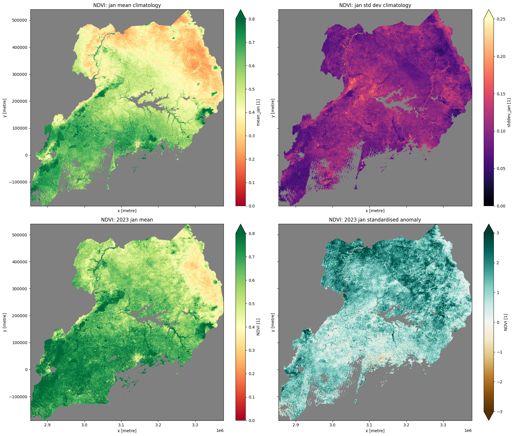
Graphique climatologique NDVI, moyenne mensuelle et anomalie standardisée
[19]:
# plot all layers
plt.rcParams["axes.facecolor"] = "gray"  # makes transparent pixels obvious
fig, ax = plt.subplots(2, 2, sharey=True, sharex=True, figsize=(18, 15))

mean_clim.plot.imshow(ax=ax[0, 0],cmap="RdYlGn",vmin=0,vmax=0.8)
ax[0, 0].set_title("NDVI: " + month + " mean climatology")

std_clim.plot.imshow(ax=ax[0, 1], cmap='magma', vmin=0, vmax=0.25)
ax[0, 1].set_title("NDVI: " + month + " std dev climatology")

month_mean.plot.imshow(ax=ax[1, 0], cmap="RdYlGn",vmin=0,vmax=0.8)
ax[1, 0].set_title("NDVI: " + year + " " + month + " mean")

stand_anomalies.plot.imshow(ax=ax[1, 1], cmap="BrBG", vmin=-3, vmax=3)
ax[1, 1].set_title("NDVI: " + year + " " + month + " standardised anomaly")
plt.tight_layout();
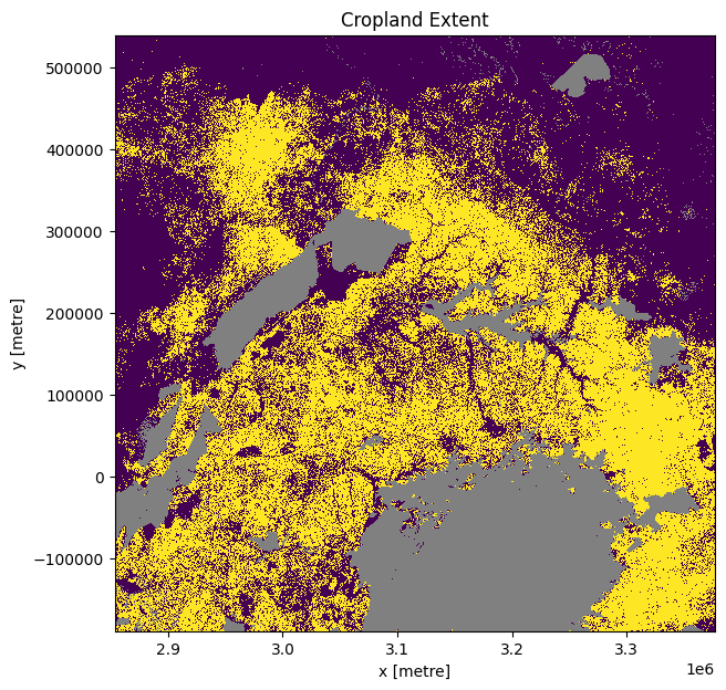
Intégration de la carte de l’étendue des terres cultivées de l’Afrique de l’Est
Chargez le masque de culture sur la région d’intérêt. La région par défaut que nous analysons est en Éthiopie, nous devons donc charger soit le produit crop_mask qui couvre l’ensemble du continent africain, soit le produit crop_mask_eastern, qui couvre les pays d’Éthiopie, du Kenya, de Tanzanie, du Rwanda et du Burundi. Si vous modifiez la région d’analyse par défaut, vous devrez peut-être charger un masque de culture différent - consultez la page docs pour en savoir plus.
[20]:
cm = dc.load(product=crop_mask,
            time=('2019'),
            measurements='mask',
            resampling='nearest',
            like=ds_ls.odc.geobox).mask.squeeze()

# convert the missing values (255) to NaN
cm = cm.where(cm != 255)

cm.plot.imshow(add_colorbar=False, figsize=(7,7))
plt.title('Cropland Extent');
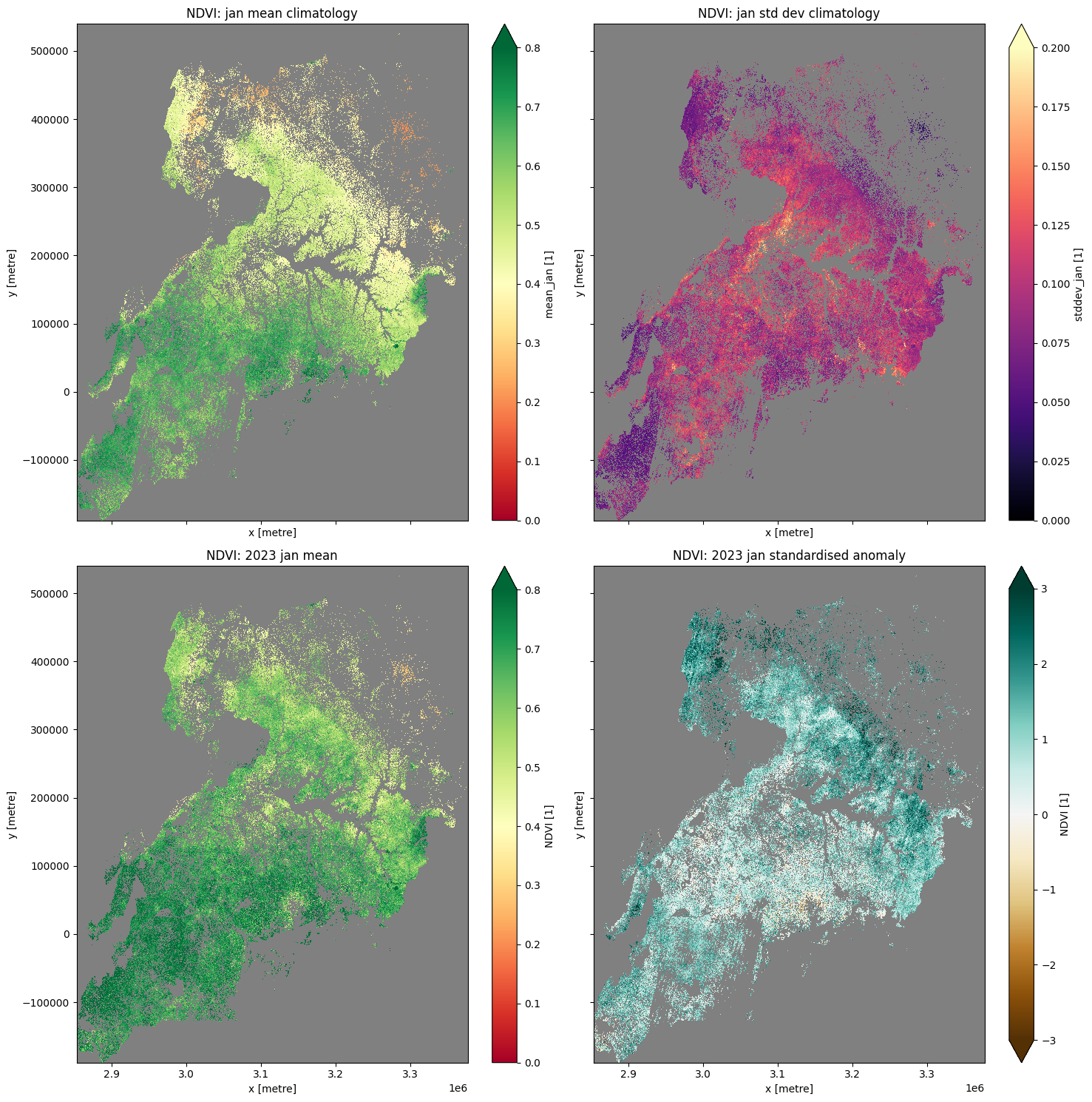
Graphique des climatologies NDVI, moyenne mensuelle et anomalies pour les régions de culture uniquement
Ci-dessous, nous masquons les régions qui ne sont pas recadrées, révélant uniquement l’état des régions recadrées.
[21]:
#mask layers with crop-mask
mean_clim_crop=mean_clim.where(cm==1, np.nan)
std_clim_crop=std_clim.where(cm==1, np.nan)
month_mean_crop=month_mean.where(cm==1, np.nan)
stand_anomalies_crop=stand_anomalies.where(cm==1, np.nan)
[22]:
#plot al layers
plt.rcParams['axes.facecolor'] = 'gray' # makes transparent pixels obvious
fig,ax = plt.subplots(2,2, sharey=True, sharex=True, figsize=(15,15))

mean_clim_crop.plot.imshow(ax=ax[0,0], cmap='RdYlGn' ,vmin=0, vmax=0.8)
ax[0,0].set_title('NDVI: '+month+' mean climatology')

std_clim_crop.plot.imshow(ax=ax[0,1], cmap='magma', vmin=0, vmax=0.2)
ax[0,1].set_title('NDVI: '+month+' std dev climatology')

month_mean_crop.plot.imshow(ax=ax[1,0], cmap="RdYlGn",vmin=0,vmax=0.8)
ax[1,0].set_title('NDVI: '+year+" "+month+' mean')

stand_anomalies_crop.plot.imshow(ax=ax[1,1], cmap='BrBG',vmin=-3, vmax=3)
ax[1,1].set_title('NDVI: '+year+" "+month+' standardised anomaly')
plt.tight_layout();
Informations Complémentaires
Licence Le code de ce notebook est sous licence Apache, version 2.0 <https://www.apache.org/licenses/LICENSE-2.0>`__.
Les données de Digital Earth Africa sont sous licence Creative Commons Attribution 4.0 <https://creativecommons.org/licenses/by/4.0/>.
Contact Si vous avez besoin d’aide, veuillez poster une question sur le canal Slack DE Africa <https://digitalearthafrica.slack.com/> ou sur le GIS Stack Exchange <https://gis.stackexchange.com/questions/ask?tags=open-data-cube> en utilisant la balise open-data-cube (vous pouvez consulter les questions posées précédemment `ici <https://gis.stackexchange.com/questions/tagged/open-data-
Si vous souhaitez signaler un problème avec ce notebook, vous pouvez en déposer un sur Github.
Version de Datacube compatible
[23]:
print(datacube.__version__)
1.9.13
Dernier test :
[24]:
from datetime import datetime
datetime.today().strftime('%Y-%m-%d')
[24]:
'2026-04-13'