Suivi de l’érosion côtière le long des côtes africaines

Produits utilisés : ls8_sr, ls9_sr s2_l2a s1_rtc

Aperçu

Plus de 40 % de la population mondiale vit à moins de 100 km du littoral. Cependant, les environnements côtiers sont en constante évolution, l’érosion et les changements côtiers représentant un défi majeur pour les infrastructures côtières précieuses et les habitats écologiques importants. Des données actualisées sur les changements côtiers et l’érosion sont essentielles pour que les gestionnaires côtiers puissent identifier et minimiser les impacts de ces changements et de cette érosion.

La surveillance des littoraux et des rivières à l’aide d’enquêtes de terrain peut s’avérer difficile et dangereuse, en particulier à l’échelle régionale ou nationale. La photographie aérienne et le LiDAR peuvent être utilisés pour surveiller l’évolution des côtes, mais cette méthode est souvent coûteuse et nécessite de nombreux vols répétés au-dessus des mêmes zones du littoral pour établir un historique précis de l’évolution du littoral au fil du temps.

Les images provenant de satellites tels que les constellations Landsat de la NASA/USGS et Copernicus Sentinel-1/2 sont disponibles gratuitement sur l’ensemble de la planète, ce qui fait de l’imagerie satellite un outil puissant et rentable pour la surveillance des côtes et des rivières à l’échelle régionale ou nationale.

Cas d’utilisation DE Afrique

L’utilité des images optiques telles que Landsat <https://docs.digitalearthafrica.org/en/latest/data_specs/Landsat_C2_SR_specs.html> et Sentinel-2 <https://docs.digitalearthafrica.org/en/latest/data_specs/Sentinel-2_Level-2A_specs.html> dans la zone côtière peut être affectée par la présence de nuages, le reflet du soleil sur l’eau, la mauvaise qualité de l’eau (par exemple les sédiments) et l’influence des marées. L’effet de ces facteurs peut être réduit en combinant des images individuelles bruyantes dans des couches « récapitulatives » ou composites plus propres, et en filtrant les données pour se concentrer uniquement sur les images prises dans certaines conditions de marée (par exemple à mi-marée). Ces images composites propres et contraintes par les marées peuvent ensuite être utilisées pour identifier et extraire la limite précise entre l’eau et la terre. Cela nous permet d’extraire des rivages précis qui peuvent être comparés dans le temps pour révéler les points chauds d’érosion et de changement côtier.

Les observations radar ne sont pas affectées par la couverture nuageuse. En développant un processus permettant de classer les pixels observés comme étant de l’eau ou de la terre, il est possible d’identifier le littoral par tous les temps à partir des données de rétrodiffusion prêtes à l’analyse Sentinel-1 <https://docs.digitalearthafrica.org/en/latest/data_specs/Sentinel-1_specs.html>. Étant donné que la mesure radar est sensible à la rugosité de la surface, à la teneur en humidité et à la géométrie de visualisation, la délimitation du littoral peut être affectée par les conditions de surface telles que les vagues déferlantes. Notre approche composite temporelle réduit le bruit causé par des conditions temporaires, mais les rivages cartographiés par radar peuvent toujours être biaisés par rapport au littoral identifié dans l’imagerie optique. Par exemple, les plages lisses et plates peuvent être confondues avec de l’eau lorsqu’elles présentent des valeurs de rétrodiffusion extrêmement faibles.

Description

Dans cet exemple, nous utilisons une version simplifiée de la méthode DE Africa Coastlines pour combiner des données de séries chronologiques avec des techniques de composition d’images et de filtrage des marées afin de cartographier avec précision les côtes au fil du temps et d’identifier les changements. Pour une zone d’intérêt sélectionnée, les données de Landsat, Sentinel-2 ou Sentinel-1 sont sélectionnées en fonction de leur disponibilité.

Les étapes suivantes sont illustrées :

Interrogez les données satellite et sélectionnez le meilleur produit disponible
Traiter les données sélectionnées et générer des images composites annuelles pour chaque année
Extraire les littoraux et calculer les taux de changement côtier

Commencer

Pour exécuter cette analyse, exécutez toutes les cellules du bloc-notes, en commençant par la cellule « Charger les packages ».

Une fois l’analyse terminée, revenez à la cellule « Paramètres d’analyse », modifiez certaines valeurs (par exemple, choisissez un autre lieu ou une autre période à analyser) et relancez l’analyse. Vous trouverez des instructions supplémentaires sur la modification du bloc-notes à la fin.

Charger des paquets

Nous devons d’abord installer des outils supplémentaires à partir du référentiel DE Africa Coastlines qui nous permettront d’estimer les taux de changement côtier. > Remarque : si vous rencontrez des messages d’erreur dans cette analyse, essayez de redémarrer le bloc-notes en cliquant sur Kernel, puis sur Redémarrer le noyau et effacer toutes les sorties.

[1]:

pip install -q git+https://github.com/digitalearthafrica/deafrica-coastlines.git@S2_test --disable-pip-version-check

Note: you may need to restart the kernel to use updated packages.

Nous pouvons maintenant charger les packages Python clés et les fonctions de support pour l’analyse.

[2]:

%matplotlib inline

import os
import warnings

import datacube
import geopandas as gpd
import matplotlib
import matplotlib.animation as animation
import matplotlib.pyplot as plt
import numpy as np
import pandas as pd
import rioxarray
import seaborn as sns
from IPython.display import Image
from matplotlib.colors import ListedColormap
from odc.geo.geom import Geometry
from skimage.filters import threshold_minimum

warnings.filterwarnings("ignore")

from coastlines.raster import load_tidal_subset, tide_cutoffs
from coastlines.vector import annual_movements, calculate_regressions, points_on_line
from deafrica_tools.areaofinterest import define_area
from deafrica_tools.bandindices import calculate_indices
from deafrica_tools.dask import create_local_dask_cluster
from deafrica_tools.datahandling import load_ard, load_best_available_ds, preprocess_s1
from deafrica_tools.plotting import display_map, rgb, xr_animation
from deafrica_tools.spatial import subpixel_contours
from eo_tides.eo import pixel_tides

Configurer un cluster Dask

Dask peut être utilisé pour mieux gérer l’utilisation de la mémoire et effectuer l’analyse en parallèle. Pour une introduction à l’utilisation de Dask avec Digital Earth Africa, consultez le Dask notebook.

Remarque : nous vous recommandons d’ouvrir la fenêtre de traitement Dask pour afficher les différents calculs en cours d’exécution ; pour ce faire, consultez la section Tableau de bord Dask en Afrique de l’Ouest du Dask notebook.

Pour utiliser Dask, configurez le cluster de calcul local à l’aide de la cellule ci-dessous.

[3]:

client = create_local_dask_cluster(return_client=True)

Client

Client-f1bb601b-c45e-11f0-8650-22be2d1047ac

Connection method: Cluster object	Cluster type: distributed.LocalCluster
Dashboard: /user/mpho.sadiki@digitalearthafrica.org/proxy/32829/status

Cluster Info

LocalCluster

4afb3ee6

Dashboard: /user/mpho.sadiki@digitalearthafrica.org/proxy/32829/status	Workers: 1
Total threads: 4	Total memory: 26.21 GiB
Status: running	Using processes: True

Scheduler Info

Scheduler

Scheduler-3055df79-a698-4a26-8528-cd7bf262e705

Comm: tcp://127.0.0.1:46569	Workers: 1
Dashboard: /user/mpho.sadiki@digitalearthafrica.org/proxy/32829/status	Total threads: 4
Started: Just now	Total memory: 26.21 GiB

Workers

Worker: 0

Comm: tcp://127.0.0.1:34915	Total threads: 4
Dashboard: /user/mpho.sadiki@digitalearthafrica.org/proxy/38429/status	Memory: 26.21 GiB
Nanny: tcp://127.0.0.1:43625
Local directory: /tmp/dask-scratch-space/worker-3dzg6jpf

Se connecter au datacube

Activez la base de données Datacube, qui fournit des fonctionnalités pour le chargement et l’affichage des données d’observation de la Terre stockées.

[4]:

dc = datacube.Datacube(app="Coastal_erosion_Landsat_Sentinel")

Paramètres d’analyse

L’ensemble de cellules suivant définit des paramètres importants pour l’analyse :

« lat » : la latitude centrale à analyser (par exemple « 14,283 »).
« lon » : la longitude centrale à analyser (par exemple « -16,921 »).
« buffer » : le nombre de degrés carrés à charger autour de la latitude et de la longitude centrales. Pour des temps de chargement raisonnables, définissez cette valeur sur « 0,1 » ou moins.
time_range : la plage de dates à analyser (par exemple ('2018', '2021'))
time_step: Ce paramètre nous permet de choisir la durée des périodes de temps que nous voulons comparer : par exemple, les littoraux pour chaque année, ou les littoraux pour chaque semestre, etc. 1Y générera un littoral pour chaque année dans l’ensemble de données ; 2Y produira un littoral pour tous les deux ans, etc.
filter_size : un nombre entier définissant la taille de la fenêtre de filtrage des taches utilisée pour Sentinel-1. Comme nous utiliserons des composites temporels, qui aideront à supprimer le bruit des taches, nous recommandons de définir cette taille de filtre sur Aucun pour désactiver le filtrage des taches, ou sur une valeur très petite (par exemple 2) pour éviter une dégradation significative de la résolution spatiale.
s1_orbit_filtering : une valeur booléenne définissant s’il faut filtrer les observations Sentinel-1 par orbite satellite. Lorsque ce paramètre est défini sur True, un filtrage par pixel sera appliqué pour conserver uniquement les observations acquises sur l’orbite avec la fréquence la plus élevée. Ce paramètre est défini sur False par défaut, ce qui signifie que les observations des orbites descendantes et ascendantes seront renvoyées.

Sélectionnez l’emplacement

Pour définir la zone d’intérêt, deux méthodes sont disponibles :

En spécifiant la latitude, la longitude et la zone tampon. Cette méthode nécessite que vous saisissiez la latitude centrale, la longitude centrale et la valeur de la zone tampon en degrés carrés autour du point central que vous souhaitez analyser. Par exemple, « lat = 10,338 », « lon = -1,055 » et « buffer = 0,1 » sélectionneront une zone avec un rayon de 0,1 degré carré autour du point avec les coordonnées (10,338, -1,055).

Vous pouvez également fournir des valeurs de tampon distinctes pour la latitude et la longitude d’une zone rectangulaire. Par exemple, « lat = 10.338 », « lon = -1.055 » et « lat_buffer = 0.1 » et « lon_buffer = 0.08 » sélectionneront une zone rectangulaire s’étendant sur 0,1 degré au nord et au sud et 0,08 degré à l’est et à l’ouest à partir du point « (10.338, -1.055) ».

Pour des temps de chargement raisonnables, définissez la mémoire tampon sur « 0,1 » ou moins.
By uploading a polygon as a GeoJSON or Esri Shapefile. If you choose this option, you will need to upload the geojson or ESRI shapefile into the Sandbox using Upload Files button in the top left corner of the Jupyter Notebook interface. ESRI shapefiles must be uploaded with all the related files (.cpg, .dbf, .shp, .shx). Once uploaded, you can use the shapefile or geojson to define the area of interest. Remember to update the code to call the file you have uploaded.

Pour utiliser l’une de ces méthodes, vous pouvez décommenter la ligne de code concernée et commenter l’autre. Pour commenter une ligne, ajoutez le symbole "#" avant le code que vous souhaitez commenter. Par défaut, la première option qui définit l’emplacement à l’aide de la latitude, de la longitude et du tampon est utilisée.

Si vous exécutez le bloc-notes pour la première fois, conservez les paramètres par défaut ci-dessous. Cela montrera comment fonctionne l’analyse et fournira des résultats significatifs. L’exemple explore les changements côtiers aux Comores.

Pour exécuter le notebook pour une zone différente, assurez-vous qu’au moins une des données Landsat, Sentinel-2 ou Sentinel-1 est disponible pour le nouvel emplacement, ce que vous pouvez vérifier sur DE Africa Explorer.

Pour garantir que la partie modélisation des marées de cette analyse fonctionne correctement, assurez-vous que une partie de la zone d’étude est située au-dessus de l’eau lors du réglage de « lat_range » et « lon_range ».

[5]:

# Define the area of interest

# Method 1: Specify the latitude, longitude, and buffer
aoi = define_area(lat=-12.27, lon=43.726, buffer=0.01)

# Method 2: Use a polygon as a GeoJSON or Esri Shapefile.
# aoi = define_area(vector_path='aoi.shp')

# Create a geopolygon and geodataframe of the area of interest
geopolygon = Geometry(aoi["features"][0]["geometry"], crs="epsg:4326")
geopolygon_gdf = gpd.GeoDataFrame(geometry=[geopolygon], crs=geopolygon.crs)

# Get the latitude and longitude range of the geopolygon
lat_range = (geopolygon_gdf.total_bounds[1], geopolygon_gdf.total_bounds[3])
lon_range = (geopolygon_gdf.total_bounds[0], geopolygon_gdf.total_bounds[2])

# Set the range of dates for the analysis, time step and tide range
time_range = ("2018", "2023")
time_step = "1Y"

# Speckle filtering size for Sentinel-1 data
filter_size = 2

# whether to apply orbit filtering
s1_orbit_filtering = True

Afficher l’emplacement sélectionné

La cellule suivante affichera la zone sélectionnée sur une carte interactive. N’hésitez pas à zoomer et dézoomer pour mieux comprendre la zone que vous allez analyser. En cliquant sur n’importe quel point de la carte, vous découvrirez les coordonnées de latitude et de longitude de ce point.

[6]:

display_map(x=lon_range, y=lat_range)

[6]:

Make this Notebook Trusted to load map: File -> Trust Notebook

Requête pour trouver le meilleur produit disponible

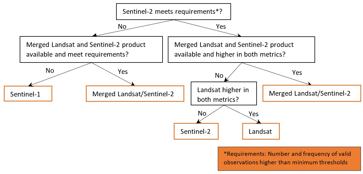
La première étape de cette analyse consiste à sélectionner parmi les produits d’imagerie satellite disponibles (Landsat, Sentinel-2, Sentinel-1 ou Landsat et Sentinel-2 fusionnés) et à charger le meilleur produit disponible pour la cartographie du littoral à l’emplacement et à la période d’étude donnés. Ici, nous utilisons la fonction load_best_available_ds pour sélectionner et charger les données. La fonction implémente quelques étapes :

Interrogez les trois produits à l’aide des fonctions « lat_range », « lon_range » et « time_range » spécifiées ci-dessus et de la fonction « load_ard ». La fonction « load_ard » chargera et masquera automatiquement les nuages de l’ensemble de données, ce qui nous permettra de nous concentrer sur les pixels contenant des données utiles. Pour plus d’informations, consultez le bloc-notes « Using load_ard <../Frequently_used_code/Using_load_ard.ipynb> »__.
Calculez le nombre moyen et la fréquence des observations valides pour chaque période. Le calcul peut éventuellement être limité à une zone côtière simplifiée au lieu de l’étendue complète de l’image.
Appliquez les règles de sélection de produits en utilisant les nombres moyens et les fréquences calculés des observations valides, en fonction de l’arbre de décision illustré dans la figure ci-dessous. Par défaut, le nombre et la fréquence requis d’observations valides dans chaque période sont respectivement de 10 et 20 %, ce qui peut également être modifié en définissant les paramètres « thresh_n_valid » et « thresh_freq ».

La fonction prend en compte les paramètres « dc », « lat_range », « lon_range », « time_range » et « time_step » comme indiqué ci-dessus. D’autres paramètres facultatifs importants incluent :

combine_ls_s2 : une valeur booléenne qui décide d’inclure ou non les produits Landsat et Sentinel-2 fusionnés parmi les produits à choisir. Par défaut, elle est définie sur False afin que seuls Landsat, Sentinel-2 ou Sentinel-1 soient utilisés.
coastal_masking : une valeur booléenne qui décide de calculer ou non un masque de zone côtière simplifié et de restreindre la comparaison des produits dans la zone masquée. L’activation de cette option exclurait probablement les pixels situés en dehors de la zone côtière (par exemple, les eaux intérieures ou profondes) qui ne sont pas essentiels à la cartographie du littoral, mais qui nécessitent plus de temps (par exemple, plusieurs minutes) pour être traités. Par défaut, ce paramètre est défini sur False pour accélérer la requête et le chargement des données.
set_resolution : une résolution spatiale prédéfinie (par exemple 20) en mètres pour interroger tous les produits. Par défaut, ce paramètre n’est pas défini, donc les résolutions d’origine des produits seront utilisées, c’est-à-dire 30 m pour Landsat, 20 m pour Sentinel-1 et 10 m pour Sentinel-2.
set_product : définissez ce paramètre pour interroger et charger uniquement un produit présélectionné, c’est-à-dire « ls » pour Landsat, « s1 » pour Sentinel-1, « s2 » pour Sentinel-2 ou « ls_s2 » pour les données fusionnées/empilées Landsat et Sentinel-2. En définissant ce paramètre, aucun autre produit ne sera interrogé ou comparé.

Remarque : selon le réglage des paramètres, la cellule ci-dessous peut prendre plus de 10 minutes pour se terminer.

[7]:

%%time
ds_selected, product_name = load_best_available_ds(
    dc, lat_range, lon_range, time_range, time_step, set_product="s2"
)

No resolution pre-set, using default resolutions for individual products...

Pre-selected product: Sentinel-2
Using pixel quality parameters for Sentinel 2
Finding datasets
    s2_l2a
Counting good quality pixels for each time step

/opt/venv/lib/python3.12/site-packages/rasterio/warp.py:387: NotGeoreferencedWarning: Dataset has no geotransform, gcps, or rpcs. The identity matrix will be returned.
  dest = _reproject(

Filtering to 637 out of 868 time steps with at least 20.0% good quality pixels
Applying morphological filters to pq mask [('opening', 2), ('dilation', 5)]
Applying pixel quality/cloud mask
Returning 637 time steps as a dask array
CPU times: user 1min 13s, sys: 7.64 s, total: 1min 20s
Wall time: 19min 48s

La fonction ci-dessus imprimera des informations utiles sur le réglage des paramètres, la progression du traitement et la raison pour laquelle le produit est choisi en fonction des règles de sélection. En utilisant les paramètres par défaut définis dans ce bloc-notes, vous constaterez que Sentinel-2 est choisi comme le meilleur produit disponible par la fonction ci-dessus, car il présente le nombre moyen et la fréquence d’observations valides les plus élevés par rapport à Landsat sur l’ensemble de la scène et à chaque pas de temps. De plus, Sentinel-2 et Landsat sont préférés à Sentinel-1 en raison des difficultés occasionnelles à distinguer la terre et l’eau dans les images de rétrodiffusion SAR. Les plages lisses et plates, en particulier, peuvent présenter des valeurs de rétrodiffusion extrêmement faibles, ce qui rend difficile la différenciation des pixels d’eau.

Si la plage de dates est définie pour commencer avant 2017, seules les données Landsat seront interrogées et chargées en raison de la disponibilité limitée des données Sentinel.

Une fois le chargement terminé, vous pouvez examiner le nom du produit et les données en les imprimant dans la cellule suivante. L’argument « Dimensions » révèle le nombre d’intervalles de temps dans l’ensemble de données, ainsi que le nombre de pixels dans les dimensions « x » (longitude) et « y » (latitude).

[8]:

print(product_name, "\n", ds_selected)

s2
 <xarray.Dataset> Size: 466MB
Dimensions:      (time: 594, y: 223, x: 220)
Coordinates:
  * time         (time) datetime64[ns] 5kB 2018-01-17T07:22:03 ... 2023-12-30...
  * y            (y) float64 2kB -1.356e+06 -1.356e+06 ... -1.358e+06 -1.358e+06
  * x            (x) float64 2kB 3.603e+05 3.604e+05 ... 3.625e+05 3.625e+05
    spatial_ref  int32 4B 32638
Data variables:
    red          (time, y, x) float32 117MB dask.array<chunksize=(1, 223, 220), meta=np.ndarray>
    green        (time, y, x) float32 117MB dask.array<chunksize=(1, 223, 220), meta=np.ndarray>
    blue         (time, y, x) float32 117MB dask.array<chunksize=(1, 223, 220), meta=np.ndarray>
    swir_1       (time, y, x) float32 117MB dask.array<chunksize=(1, 223, 220), meta=np.ndarray>
Attributes:
    crs:           epsg:32638
    grid_mapping:  spatial_ref

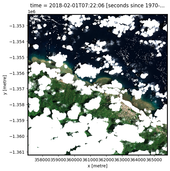
Exemple d’horodatage de tracé

Ici, nous pouvons tracer un exemple d’image à l’emplacement sélectionné à un horodatage donné. Pour visualiser les données Landsat ou Sentinel-2, utilisez la fonction utilitaire préchargée « rgb » pour tracer une image en vraies couleurs pour un horodatage donné. Les zones blanches indiquent où les nuages ou d’autres pixels non valides de l’image ont été masqués. Si le produit sélectionné est Sentinel-1, nous traçons la bande vh comme exemple.

[9]:

# Set the timesteps to visualise
timestamp = 4
if (product_name == "ls") or (product_name == "s2") or (product_name == "ls_s2"):
    # Generate RGB plots at each timestep
    rgb(ds_selected, index=timestamp, percentile_stretch=[0, 0.999])
else:
    ds_selected["vh"].isel(time=timestamp).plot.imshow(robust=True)

../../../_images/sandbox_notebooks_Real_world_examples_Coastal_erosion_22_0.png

Modifiez la valeur de « timestamp » et réexécutez la cellule pour tracer un horodatage différent (les horodatages sont numérotés de « 0 » à « n_time - 1 » où « n_time » est le nombre total d’horodatages ; voir la liste « time » sous la catégorie « Dimensions » dans l’impression du jeu de données ci-dessus).

Traiter les données sélectionnées et générer des composites annuels

Modèle de hauteur de marée

For each satellite timestep, we use the pixel_tides function from the `eo-tides <https://geoscienceaustralia.github.io/eo-tides/>`__ Python package to model tide heights (EOT20 model by default) into a low-resolution 5 x 5 km grid, then reprojects modelled tides into the spatial extent of our satellite image. We add this new data as a new variable tide_height in our satellite dataset to allow each satellite pixel to be analysed and filtered/masked based on the tide height at the exact moment of satellite image acquisition.

[10]:

ds_selected["tide_height"] = pixel_tides(data=ds_selected,  directory="/var/share/tide_models", resample=True)

Creating reduced resolution 5000 x 5000 metre tide modelling array
Modelling tides with EOT20
Reprojecting tides into original resolution

Sur la base de l’ensemble des séries chronologiques des hauteurs de marée, nous pouvons calculer la hauteur de marée maximale et minimale observée par satellite pour chaque pixel, puis calculer les seuils de marée utilisés pour restreindre nos données aux observations par satellite centrées sur la marée moyenne (0 m au-dessus du niveau moyen de la mer) à l’aide de la fonction tide_cutoffs :

[11]:

# Determine tide cutoff
tide_cutoff_min, tide_cutoff_max = tide_cutoffs(
    ds_selected, ds_selected["tide_height"], tide_centre=0.0
)

Les seuils de marée étant calculés pour tous les pixels, nous ne conservons désormais que les observations comprises dans les plages de seuils de hauteur de marée. Nous souhaitons également supprimer les pas de temps sans pixels compris dans les plages de seuils :

[12]:

tide_bool = (ds_selected.tide_height >= tide_cutoff_min) & (
    ds_selected.tide_height <= tide_cutoff_max
)
ds_selected = ds_selected.sel(time=tide_bool.sum(dim=["x", "y"]) > 0)

# Apply mask, and load in corresponding tide masked data
ds_selected = ds_selected.where(tide_bool)
print(ds_selected)

<xarray.Dataset> Size: 308MB
Dimensions:      (time: 314, y: 223, x: 220)
Coordinates:
  * time         (time) datetime64[ns] 3kB 2018-01-22T07:22:04 ... 2023-12-22...
  * y            (y) float64 2kB -1.356e+06 -1.356e+06 ... -1.358e+06 -1.358e+06
  * x            (x) float64 2kB 3.603e+05 3.604e+05 ... 3.625e+05 3.625e+05
    spatial_ref  int32 4B 32638
    tide_model   <U5 20B 'EOT20'
Data variables:
    red          (time, y, x) float32 62MB dask.array<chunksize=(1, 223, 220), meta=np.ndarray>
    green        (time, y, x) float32 62MB dask.array<chunksize=(1, 223, 220), meta=np.ndarray>
    blue         (time, y, x) float32 62MB dask.array<chunksize=(1, 223, 220), meta=np.ndarray>
    swir_1       (time, y, x) float32 62MB dask.array<chunksize=(1, 223, 220), meta=np.ndarray>
    tide_height  (time, y, x) float32 62MB -0.1426 -0.1426 ... 0.3011 0.3011
Attributes:
    crs:           epsg:32638
    grid_mapping:  spatial_ref

Traiter les données sélectionnées

Pour extraire les emplacements des côtes, nous devons être capables de séparer l’eau de la terre dans notre zone d’étude. Pour ce faire, pour Landsat ou Sentinel-2, nous pouvons calculer un indice d’eau appelé « Modified Normalised Difference Water Index », ou MNDWI. Cet indice utilise le rapport entre le rayonnement vert et le rayonnement infrarouge à ondes courtes (SWIR) pour identifier la présence d’eau (Xu 2006) <https://doi.org/10.1080/01431160600589179>. La formule est :

\[\begin{aligned} \text{MNDWI} &= \frac{(\text{Vert} - \text{SWIR})}{(\text{Vert} + \text{SWIR})} \end{aligned}\]

où « Vert » est la bande verte et « SWIR » est la bande SWIR.

Pour les données Sentinel-1, nous avons implémenté quelques étapes de prétraitement facultatives. Comme les observations radar apparaissent mouchetées en raison de l’interférence aléatoire de signaux cohérents provenant de la diffusion des cibles, nous avons implémenté un filtrage des mouchetures à l’aide du filtre Lee, l’un des filtres de mouchetures adaptatifs les plus populaires qui prend en compte l’homogénéité locale.

De plus, chacune des observations de Sentinel-1 a été acquise à partir d’une orbite descendante ou ascendante. La direction orbitale a un impact sur l’angle d’incidence local et la valeur de rétrodiffusion. Par conséquent, nous avons mis en œuvre un filtrage par pixel pour ne conserver que les observations de l’orbite dominante, ce qui devrait minimiser les effets d’un angle de visée et d’une direction d’obit incohérents pour chaque pixel individuel. De plus, il est souvent utile de convertir la rétrodiffusion en décibels (dB) pour l’analyse. La rétrodiffusion en dB a un profil de bruit plus symétrique et une distribution de valeurs moins biaisée pour une évaluation statistique plus facile.

Ces étapes de prétraitement sont appliquées à l’aide de la fonction « preprocess_s1 » et des paramètres « filter_size » et « s1_orbit_filtering » comme spécifié au début du bloc-notes. Notez que le prétraitement de Sentinel-1 peut prendre quelques minutes.

[13]:

if product_name == "ls":
    # Calculate the water index
    ds_selected = calculate_indices(ds_selected, index="MNDWI", satellite_mission="ls")
elif (product_name == "s2") or (product_name == "ls_s2"):
    # Calculate the water index
    ds_selected = calculate_indices(ds_selected, index="MNDWI", satellite_mission="s2")
else:
    ds_selected = preprocess_s1(
        ds_selected, filter_size=filter_size, s1_orbit_filtering=s1_orbit_filtering
    )

Combinez les observations dans des images récapitulatives sans bruit

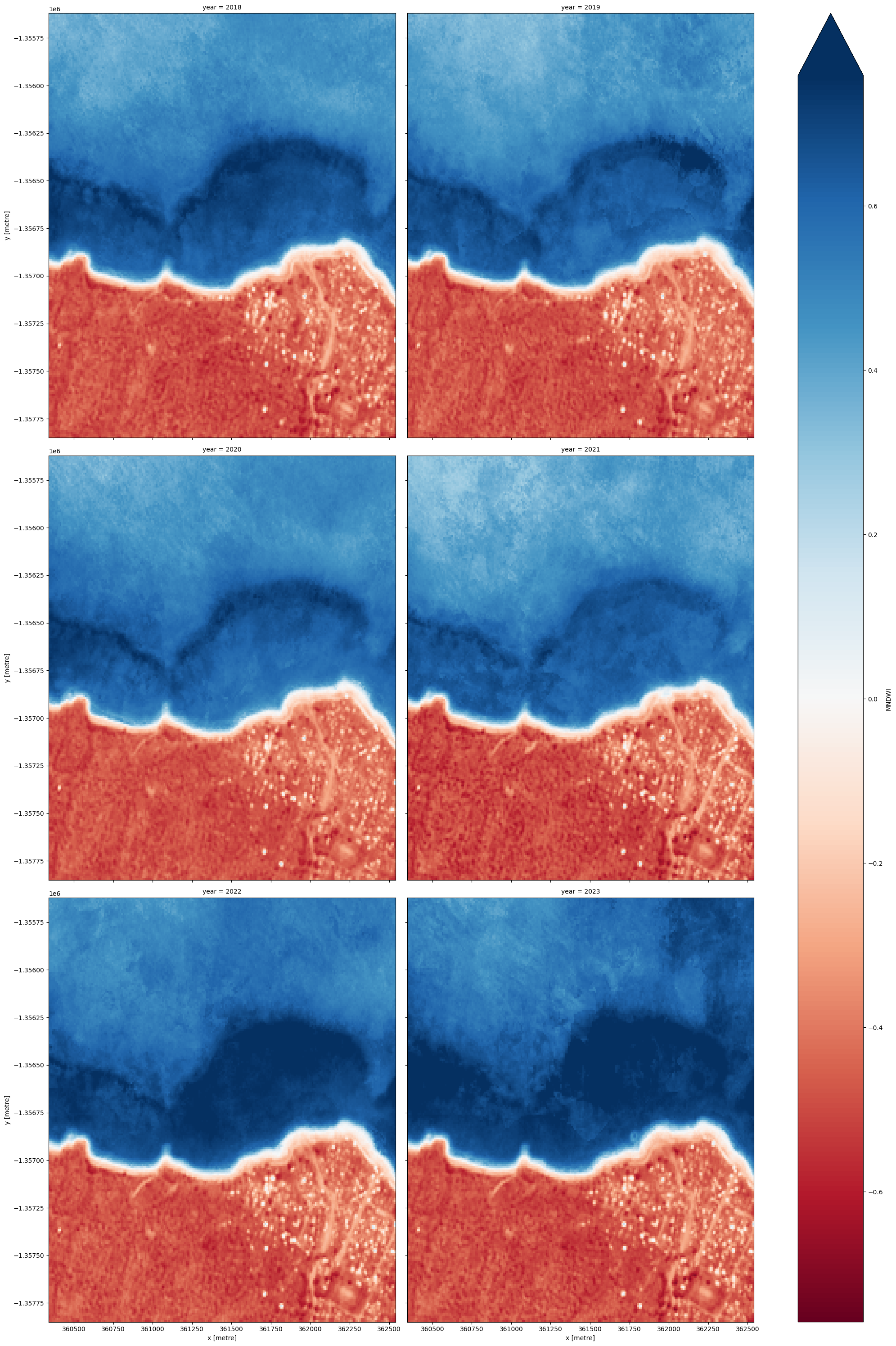
Les images de télédétection individuelles peuvent être affectées par des données bruyantes, par exemple les nuages/ombres de nuages pour les images optiques et les effets du vent sur l’eau pour les images radar. Pour produire des images plus nettes qui peuvent être comparées plus facilement dans le temps, nous pouvons créer des images « récapitulatives » ou composites qui combinent plusieurs images en une seule image pour révéler la médiane ou l’apparence « typique » du paysage pour une certaine période. Dans ce cas, nous utilisons la médiane comme statistique récapitulative car elle empêche les valeurs aberrantes de fausser les données, ce qui ne serait pas le cas si nous devions utiliser la moyenne.

Dans le code ci-dessous, nous prenons la série chronologique d’images et les combinons en images uniques pour chaque « time_step ». Par exemple, si « time_step = “1Y” », le code produira une nouvelle image pour chaque année de l’ensemble de données. Cette étape peut prendre plusieurs minutes à charger si la zone d’étude est vaste.

Remarque : nous vous recommandons d’ouvrir la fenêtre de traitement Dask pour afficher les différents calculs en cours d’exécution ; pour ce faire, consultez la section Tableau de bord Dask en Afrique de l’Ouest du Dask notebook.

Lorsqu’il s’agit d’interpréter l’indice, les valeurs élevées (couleurs bleues) représentent généralement les pixels d’eau, tandis que les valeurs faibles (couleurs rouges) représentent la terre.

[14]:

# Combine into summary images by `time_step`
if (product_name == "ls") or (product_name == "s2") or (product_name == "ls_s2"):
    var = "MNDWI"
else:
    var = "vh"

ds_summaries = ds_selected[[var]].resample(time=time_step).median("time").compute()
# Rename time attribute as year
ds_summaries["time"] = ds_summaries.time.dt.year
ds_summaries = ds_summaries.rename(time="year")

# Plot the output summary images
ds_summaries[var].plot(col="year", cmap="RdBu", col_wrap=2, robust=True, size=10)
plt.show()

../../../_images/sandbox_notebooks_Real_world_examples_Coastal_erosion_34_0.png

[15]:

# Shut down Dask client now that we have processed the data we need
client.close()

Extraire les littoraux et calculer les taux de changement côtier

Extraire les rivages à partir d’images

Nous souhaitons maintenant extraire un littoral précis pour chacune des images récapitulatives ci-dessus. Le code ci-dessous identifie la limite entre la terre et l’eau en traçant une ligne le long des pixels avec une valeur de seuil donnée. Pour les images Landsat et Sentinel-2, nous utilisons une valeur d’indice d’eau de « 0 ».

Pour les images Sentinel-1, le seuil peut être déterminé soit par un simple seuillage automatique, soit à l’aide d’une méthode de classification supervisée plus complexe. Dans ce notebook, nous utilisons la fonction threshold_minimum, qui calcule l’histogramme pour toutes les valeurs de rétrodiffusion, le lisse jusqu’à ce qu’il n’y ait que deux maxima et trouve le minimum entre les deux comme seuil.

Nous utilisons la fonction « subpixel_contours » pour identifier la limite entre la terre et l’eau en traçant une ligne le long des pixels avec la valeur de seuil précédemment identifiée. Elle renvoie un fichier vectoriel avec une ligne pour chaque pas de temps :

[16]:

if (product_name == "ls") or (product_name == "s2") or (product_name == "ls_s2"):
    threshold = 0
else:
    threshold = threshold_minimum(
        ds_selected[var].values[~np.isnan(ds_selected[var].values)]
    )

contour_gdf = subpixel_contours(
    da=ds_summaries[var],
    z_values=threshold,
    dim="year",
    crs=ds_summaries.geobox.crs,
    output_path="annual_shorelines_{}.geojson".format(product_name),
    min_vertices=15,
)
contour_gdf = contour_gdf.set_index("year")
# Preview shoreline data
contour_gdf

Operating in single z-value, multiple arrays mode
Writing contours to annual_shorelines_s2.geojson

[16]:

	geometry
year
2018	MULTILINESTRING ((362535 -1357104.58, 362526.4...
2019	MULTILINESTRING ((362535 -1357094.728, 362525 ...
2020	MULTILINESTRING ((362535 -1357109.559, 362531....
2021	MULTILINESTRING ((362535 -1357079.425, 362530....
2022	MULTILINESTRING ((362535 -1357096.093, 362534....
2023	MULTILINESTRING ((362535 -1357089.159, 362531....

Tracer des rivages rééchantillonnés sur une carte interactive

La cellule suivante fournit une carte interactive avec une superposition des rivages identifiés dans la cellule précédente. Exécutez-la pour visualiser la carte (cette étape peut prendre plusieurs minutes à charger si la zone d’étude est grande).

Zoomez sur la carte ci-dessous pour explorer l’ensemble des rivages obtenus. Les rivages les plus anciens sont colorés en noir et les rivages les plus récents en jaune. Passez la souris sur les lignes pour voir la période de temps pour chaque rivage imprimée au-dessus de la carte. Grâce à ces données, nous pouvons facilement identifier les zones du littoral ou des rivières qui ont considérablement changé au fil du temps, ou les zones qui sont restées stables pendant toute la période.

[17]:

# Plot shorelines on interactive map
bounds = np.arange(2018, 2022, 1)

contour_gdf.reset_index().explore(
    column="year",
    cmap="inferno",
    categorical=True,
    tiles="https://server.arcgisonline.com/ArcGIS/rest/services/World_Imagery/MapServer/tile/{z}/{y}/{x}",
    attr="ESRI WorldImagery",
)

[17]:

Make this Notebook Trusted to load map: File -> Trust Notebook

Calculer les taux de changement côtier

Pour identifier les parties du littoral qui évoluent rapidement, nous pouvons utiliser nos données annuelles sur le littoral pour calculer les taux de changement côtier en mètres par an. Cela peut être particulièrement utile pour révéler les points chauds de recul côtier (par exemple, l’érosion) ou les points chauds de croissance côtière.

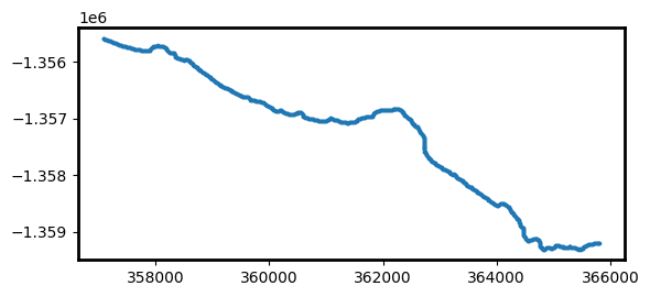
Pour ce faire, nous devons d’abord créer un ensemble de points régulièrement espacés tous les 20 mètres le long du littoral le plus récent de notre ensemble de données. Ces points seront utilisés pour tracer les taux de changement côtier dans notre zone d’étude.

[18]:

# Extract points at every 30 metres along the most recent shoreline
points_gdf = points_on_line(contour_gdf, index=2023, distance=20)
points_gdf.plot(markersize=3)

[18]:

<Axes: >

../../../_images/sandbox_notebooks_Real_world_examples_Coastal_erosion_41_1.png

Maintenant que nous disposons d’un ensemble de points de modélisation, nous pouvons mesurer les distances entre chacun des points et chaque rivage annuel. Cela nous donne un tableau de distances, où les valeurs négatives (par exemple « -6,5 ») indiquent qu’un rivage annuel était situé à l’intérieur des terres par rapport à nos points, et les valeurs positives (par exemple « 2,3 ») indiquent qu’un rivage était situé vers l’océan. Étant donné que nos points ont été créés le long de notre rivage le plus récent de 2023, les distances pour 2023 auront toujours une distance de 0 m.

[19]:

# For each 30 m-spaced point, calculate the distance from
# the most recent 2023 shoreline to each other annual shoreline
# in the datasets.
points_gdf = annual_movements(
    points_gdf,
    contours_gdf=contour_gdf,
    yearly_ds=ds_summaries,
    baseline_year=2023,
    water_index=var,
)
points_gdf

[19]:

	geometry	dist_2018	dist_2019	dist_2020	dist_2021	dist_2022	dist_2023	angle_mean	angle_std
0	POINT (362535 -1357089.159)	-10.29	-4.23	-11.64	9.73	-3.72	0.0	36	25
1	POINT (362524.022 -1357072.536)	-12.22	-7.55	-9.89	4.77	-3.11	0.0	57	22
2	POINT (362515.427 -1357054.774)	-14.54	-10.43	-12.32	1.29	-3.09	0.0	55	22
3	POINT (362505.424 -1357037.87)	-14.63	-10.40	-10.75	-0.11	-3.11	0.0	51	20
4	POINT (362494.492 -1357021.25)	-14.92	-9.00	-12.44	1.70	-2.56	0.0	55	22
...	...	...	...	...	...	...	...	...	...
124	POINT (360430.432 -1356920.401)	-3.05	-2.18	-1.75	1.53	-1.89	0.0	157	12
125	POINT (360415.676 -1356933.771)	0.19	0.26	2.09	0.80	-1.45	0.0	146	17
126	POINT (360396.536 -1356936.727)	-1.62	0.86	-0.09	0.84	-1.45	0.0	3	2
127	POINT (360377.006 -1356932.488)	-3.39	-2.18	-4.58	-0.72	-1.88	0.0	4	9
128	POINT (360357.213 -1356929.716)	-3.28	-0.52	-3.17	1.92	0.88	0.0	11	7

129 rows × 9 columns

Enfin, nous pouvons calculer les taux annuels de changement côtier (en mètres par an) à l’aide d’une régression linéaire. Cela ajoutera plusieurs nouvelles colonnes à notre tableau :

rate_time : taux de variation annuels (en mètres par an) calculés en effectuant une régression linéaire des distances annuelles du littoral en fonction du temps (à l’exclusion des valeurs aberrantes ; voir outl_time). Les valeurs négatives indiquent un recul et les valeurs positives indiquent une croissance.
« sig_time » : signification (valeur p) de la relation linéaire entre les distances annuelles du littoral et le temps. De faibles valeurs (par exemple, une valeur p < 0,01 ou 0,05) peuvent indiquer qu’un littoral subit des changements côtiers constants au fil du temps.
se_time : erreur standard (en mètres) de la relation linéaire entre les distances annuelles du littoral et le temps. Cela peut être utilisé pour générer des intervalles de confiance autour du taux de changement donné par rate_time (par exemple, intervalle de confiance à 95 % = se_time * 1,96)
outl_time : les lignes de côte annuelles individuelles sont des estimateurs bruyants de la position du littoral qui peuvent être influencés par les conditions environnementales (par exemple, les nuages, les vagues déferlantes, les embruns) ou les problèmes de modélisation (par exemple, de mauvais résultats de modélisation des marées ou des observations satellites claires limitées). Pour obtenir des taux de changement fiables, les lignes de côte aberrantes sont exclues à l’aide d’un algorithme robuste de détection des valeurs aberrantes de l’écart absolu médian et enregistrées dans cette colonne.

[20]:

# Calculate rates of change using linear regression
points_gdf = calculate_regressions(points_gdf=points_gdf, contours_gdf=contour_gdf)
points_gdf

[20]:

	rate_time	sig_time	se_time	outl_time	dist_2018	dist_2019	dist_2020	dist_2021	dist_2022	dist_2023	angle_mean	angle_std	geometry
0	2.124	0.298	1.777		-10.29	-4.23	-11.64	9.73	-3.72	0.0	36	25	POINT (362535 -1357089.159)
1	2.545	0.091	1.150		-12.22	-7.55	-9.89	4.77	-3.11	0.0	57	22	POINT (362524.022 -1357072.536)
2	3.095	0.029	0.933		-14.54	-10.43	-12.32	1.29	-3.09	0.0	55	22	POINT (362515.427 -1357054.774)
3	3.019	0.013	0.702		-14.63	-10.40	-10.75	-0.11	-3.11	0.0	51	20	POINT (362505.424 -1357037.87)
4	3.087	0.037	1.001		-14.92	-9.00	-12.44	1.70	-2.56	0.0	55	22	POINT (362494.492 -1357021.25)
...	...	...	...	...	...	...	...	...	...	...	...	...	...
124	0.554	0.190	0.352		-3.05	-2.18	-1.75	1.53	-1.89	0.0	157	12	POINT (360430.432 -1356920.401)
125	-0.211	0.506	0.289		0.19	0.26	2.09	0.80	-1.45	0.0	146	17	POINT (360415.676 -1356933.771)
126	0.060	0.845	0.287		-1.62	0.86	-0.09	0.84	-1.45	0.0	3	2	POINT (360396.536 -1356936.727)
127	0.620	0.130	0.326		-3.39	-2.18	-4.58	-0.72	-1.88	0.0	4	9	POINT (360377.006 -1356932.488)
128	0.734	0.166	0.434		-3.28	-0.52	-3.17	1.92	0.88	0.0	11	7	POINT (360357.213 -1356929.716)

129 rows × 13 columns

Tracez les taux de changement côtier sur une carte interactive

Maintenant que nous avons calculé les taux de changement côtier, nous pouvons les tracer sur une carte interactive pour identifier les parties du littoral qui reculent ou croissent au fil du temps.

Lorsque la carte ci-dessous apparaît, passez votre souris sur les points colorés qui apparaissent le long du littoral pour obtenir un résumé des changements côtiers récents à ces endroits. Les points rouges représentent les endroits en recul (par exemple, l’érosion) et les points bleus représentent les endroits en croissance.

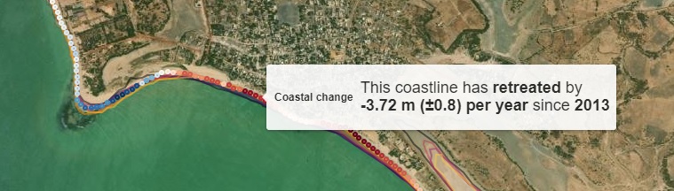
[21]:

# Add human-friendly label for plotting
points_gdf["Coastal change"] = points_gdf.apply(
    lambda x: f'<h4>This coastline has {"<b>retreated</b>" if x.rate_time < 0 else "<b>grown</b>"} '
    f"by</br><b>{x.rate_time:.2f} m (±{x.se_time:.1f}) per year</b> since "
    f"<b>{contour_gdf.index[0]}</b></h4>",
    axis=1,
)
points_gdf.loc[points_gdf.sig_time > 0.05, "Coastal change"] = (
    f"<h4>No significant trend of retreat or growth)</h4>"
)

# Add annual shorelines to map
m = contour_gdf.reset_index().explore(
    column="year",
    cmap="inferno",
    tiles="https://server.arcgisonline.com/ArcGIS/rest/services/World_Imagery/MapServer/tile/{z}/{y}/{x}",
    tooltip=False,
    style_kwds={"opacity": 0.5},
    attr="ESRI WorldImagery",
    categorical=True,
)

# Add rates of change to map
points_gdf.explore(
    m=m, column="rate_time", vmin=-5, vmax=5, tooltip="Coastal change", cmap="RdBu"
)

[21]:

Make this Notebook Trusted to load map: File -> Trust Notebook

Remarque importante : ce carnet de notes peut produire des taux de changement trompeurs pour les plans d’eau non côtiers qui peuvent fluctuer naturellement d’une année à l’autre. Le référentiel complet « Digital Earth Africa Coastlines » <https://github.com/digitalearthafrica/deafrica-coastlines.git> contient des méthodes supplémentaires pour produire des taux de changement plus précis en nettoyant et en filtrant les données annuelles sur le littoral pour se concentrer uniquement sur les littoraux côtiers.

Exporter les taux de changement vers le fichier

Enfin, nous pouvons exporter notre fichier de taux de changement de sortie afin qu’il puisse être chargé dans un logiciel SIG (par exemple ESRI ArcGIS ou QGIS).

[22]:

points_gdf.to_crs("EPSG:4326").to_file(
    "rates_of_changes_{}.geojson".format(product_name)
)

GIF animé annuel des rivages du tracé

[23]:

gdf = gpd.GeoDataFrame(
    data=contour_gdf.reset_index(), geometry=contour_gdf.reset_index().geometry
)
gdf_year = gdf.year.values

# Extract annual RGB noise-free summary images
ds_rgb = (
    ds_selected[["red", "green", "blue"]]
    .resample(time=time_step)
    .median("time")
    .compute()
)
extent = gdf.total_bounds
ds_rgb = ds_rgb.rio.clip_box(*extent)


fig, ax = plt.subplots(figsize=(15, 3))

# Generating the color scheme based on the number of years
lenyear = len(gdf_year)
palette = list((sns.color_palette("inferno", lenyear).as_hex()))
wsf = []
color = []
color_index = 0

for i in range(0, len(gdf_year)):
    year_list = gdf_year[i]
    color.append(palette[color_index])
    color_index += 1


def update(i):
    cs_plt = gdf.where(gdf.year == gdf_year[i]).plot(
        cmap=ListedColormap(palette[i]), ax=ax
    )
    t = ax.set_title(gdf_year[i], size="x-large", weight="bold")
    return cs_plt


rgb(ds_rgb, index=1, ax=ax)
ani = animation.FuncAnimation(fig, update, len(gdf_year - 1), interval=1000)
ani.save("coastline.gif")
plt.close()

Image(filename="coastline.gif")

[23]:

<IPython.core.display.Image object>

Prochaines étapes

Une fois terminé, revenez à la cellule « Configurer l’analyse », modifiez certaines valeurs (par exemple, « time_range », « time_step » ou « lat »/« lon ») et relancez l’analyse. Si vous souhaitez modifier l’emplacement, vous devrez vous assurer qu’au moins un des produits Landsat, Sentinel-2 et Sentinel-1 est disponible pour le nouvel emplacement, ce que vous pouvez vérifier sur le site DE Africa Explorer <https://explorer.digitalearth.africa/products/>`__.

Pour plus d’informations sur la méthode utilisée pour ce carnet, lisez l’article scientifique : > Bishop-Taylor, R., Nanson, R., Sagar, S., Lymburner, L. (2021). Cartographie du littoral dynamique de l’Australie au niveau moyen de la mer à l’aide de trois décennies d’images Landsat. Télédétection de l’environnement 267, 112734. Disponible : https://doi.org/10.1016/j.rse.2021.112734

Informations Complémentaires

Licence Le code de ce notebook est sous licence Apache, version 2.0 <https://www.apache.org/licenses/LICENSE-2.0>`__.

Les données de Digital Earth Africa sont sous licence Creative Commons Attribution 4.0 <https://creativecommons.org/licenses/by/4.0/>.

Contact Si vous avez besoin d’aide, veuillez poster une question sur le canal Slack DE Africa <https://digitalearthafrica.slack.com/> ou sur le GIS Stack Exchange <https://gis.stackexchange.com/questions/ask?tags=open-data-cube> en utilisant la balise open-data-cube (vous pouvez consulter les questions posées précédemment `ici <https://gis.stackexchange.com/questions/tagged/open-data-

Si vous souhaitez signaler un problème avec ce notebook, vous pouvez en déposer un sur Github.

Version de Datacube compatible

[24]:

print(datacube.__version__)

1.8.20

Dernier test :

[25]:

from datetime import datetime

datetime.today().strftime("%Y-%m-%d")

[25]:

'2025-11-18'