Surveillance de la qualité de l’eau

• Produits utilisés : ls8_sr, wofs_ls

Mots clés données utilisées ; landsat 8, données utilisées ; WOfS, méthodes de données ; composition, dask, qualité de l’eau

Aperçu

L’indicateur ODD 6.3.2 de l’ONU est la « proportion de masses d’eau dont l’eau ambiante est de bonne qualité ». Il existe de nombreuses façons de mesurer la qualité de l’eau à l’aide d’algorithmes basés sur la télédétection ; ce carnet compare plusieurs d’entre eux. Ils estiment généralement la quantité de matières en suspension dans l’eau.

Description

Ce carnet présente les résultats de trois algorithmes empiriques et d’un indice spectral traitant de la matière en suspension totale (MST) dans l’eau. Il y a un certain nombre de mises en garde à prendre en compte lors de l’application de ces algorithmes :

• Ces algorithmes ont été développés pour des régions spécifiques du monde et ne sont pas nécessairement universellement valables.

• Les données Landsat-8 sont un produit de réflectance de surface et, comme l’eau a une très faible radiance, la précision des résultats peut être considérablement affectée par de petites différences dans les conditions atmosphériques ou par des différences dans les algorithmes de correction atmosphérique.

• Les barres de couleurs de ces résultats ont été supprimées pour éviter d’afficher des quantités spécifiques pour les résultats TSM. Il est préférable d’utiliser ces résultats pour évaluer les changements qualitatifs de la qualité de l’eau (par exemple, faible, moyenne, élevée). Grâce aux améliorations apportées aux données prêtes à l’analyse (par exemple, la radiance de sortie de l’eau) et à l’échantillonnage in situ des plans d’eau pour la modélisation empirique, il sera possible d’augmenter la précision de ces résultats sur la qualité de l’eau et même de prendre en compte la sortie numérique.

Les algorithmes de qualité de l’eau présentés sont :

1. Matières en suspension totales (MST) Lymburner

2. Modèle de particules en suspension (SPM)

3. Indice de différence normalisée des sédiments en suspension (NDSSI)

4. Matières en suspension totales (MES) de Quang

---

Commencer

Pour exécuter cette analyse, exécutez toutes les cellules du bloc-notes, en commençant par la cellule « Charger les packages ».

Charger des paquets

Importez les packages Python utilisés pour l’analyse.

%matplotlib inline

import datacube
import numpy as np
import xarray as xr
import geopandas as gpd
import matplotlib.pyplot as plt
from odc.geo.geom import Geometry

from deafrica_tools.plotting import display_map, rgb
from deafrica_tools.datahandling import load_ard, mostcommon_crs, wofs_fuser
from deafrica_tools.areaofinterest import define_area

Se connecter au datacube

Activez la base de données Datacube, qui fournit des fonctionnalités pour le chargement et l’affichage des données d’observation de la Terre stockées.

dc = datacube.Datacube(app="Monitoring_water_quality")

Paramètres d’analyse

La cellule suivante définit des paramètres importants pour l’analyse. Les paramètres sont :

• « lat » : la latitude centrale à analyser (par exemple « 10,338 »).

• « lon » : la longitude centrale à analyser (par exemple « -1,055 »).

• lat_buffer : le nombre de degrés à charger autour de la latitude centrale.

• « lon_buffer » : le nombre de degrés à charger autour de la longitude centrale.

• time_range : la plage horaire à analyser, au format AAAA-MM-JJ (par exemple, ('2016-01-01', '2016-12-31')).

Si vous exécutez le bloc-notes pour la première fois, conservez les paramètres par défaut ci-dessous. Cela montrera comment fonctionne l’analyse et fournira des résultats significatifs. L’exemple porte sur la qualité de l’eau du lac Manyara.

Pour exécuter le carnet pour une zone différente, assurez-vous que les données Landsat 8 sont disponibles pour la zone choisie à l’aide de DEAfrica Explorer. Utilisez le menu déroulant pour cocher Landsat 8 (ls8_sr).

Zones suggérées

Voici quelques suggestions de zones à examiner. Pour afficher l’une de ces zones, copiez et collez les valeurs des paramètres dans la cellule ci-dessous, puis exécutez le bloc-notes.

Lac Manyara, Tanzanie

lat = -3.611
lon = 35.8261
lat_buffer = 0.2025
lon_buffer = 0.1025

Réservoir de Weija, Ghana

lat = 5.583
lon = -0.366
lat_buffer = 0.042
lon_buffer = 0.038

Lac Sulunga, Tanzanie

lat = -6.06
lon = 35.17
lat_buffer = 0.2
lon_buffer = 0.19

Sélectionnez l’emplacement

Pour définir la zone d’intérêt, deux méthodes sont disponibles :

1. En spécifiant la latitude, la longitude et la zone tampon. Cette méthode nécessite que vous saisissiez la latitude centrale, la longitude centrale et la valeur de la zone tampon en degrés carrés autour du point central que vous souhaitez analyser. Par exemple, « lat = 10,338 », « lon = -1,055 » et « buffer = 0,1 » sélectionneront une zone avec un rayon de 0,1 degré carré autour du point avec les coordonnées (10,338, -1,055).

   Vous pouvez également fournir des valeurs de tampon distinctes pour la latitude et la longitude d’une zone rectangulaire. Par exemple, « lat = 10.338 », « lon = -1.055 » et « lat_buffer = 0.1 » et « lon_buffer = 0.08 » sélectionneront une zone rectangulaire s’étendant sur 0,1 degré au nord et au sud et 0,08 degré à l’est et à l’ouest à partir du point « (10.338, -1.055) ».

   Pour des temps de chargement raisonnables, définissez la mémoire tampon sur « 0,1 » ou moins.

2. By uploading a polygon as a GeoJSON or Esri Shapefile. If you choose this option, you will need to upload the geojson or ESRI shapefile into the Sandbox using Upload Files button in the top left corner of the Jupyter Notebook interface. ESRI shapefiles must be uploaded with all the related files (.cpg, .dbf, .shp, .shx). Once uploaded, you can use the shapefile or geojson to define the area of interest. Remember to update the code to call the file you have uploaded.

Pour utiliser l’une de ces méthodes, vous pouvez décommenter la ligne de code concernée et commenter l’autre. Pour commenter une ligne, ajoutez le symbole "#" avant le code que vous souhaitez commenter. Par défaut, la première option qui définit l’emplacement à l’aide de la latitude, de la longitude et du tampon est utilisée.

# Method 1: Specify the latitude, longitude, and buffer
aoi = define_area(lat=-3.611, lon=35.8261 , lat_buffer = 0.2025, lon_buffer = 0.1025)

# Method 2: Use a polygon as a GeoJSON or Esri Shapefile.
#aoi = define_area(vector_path='aoi.shp')

#Create a geopolygon and geodataframe of the area of interest
geopolygon = Geometry(aoi["features"][0]["geometry"], crs="epsg:4326")
geopolygon_gdf = gpd.GeoDataFrame(geometry=[geopolygon], crs=geopolygon.crs)

# Get the latitude and longitude range of the geopolygon
lat_range = (geopolygon_gdf.total_bounds[1], geopolygon_gdf.total_bounds[3])
lon_range = (geopolygon_gdf.total_bounds[0], geopolygon_gdf.total_bounds[2])

# Time period
time_range = ("2016-02-16")

Afficher l’emplacement sélectionné

La cellule suivante affichera la zone sélectionnée sur une carte interactive. N’hésitez pas à zoomer et dézoomer pour mieux comprendre la zone que vous allez analyser. En cliquant sur n’importe quel point de la carte, vous découvrirez les coordonnées de latitude et de longitude de ce point.

# The code below renders a map that can be used to view the region.
display_map(lon_range, lat_range)

Make this Notebook Trusted to load map: File -> Trust Notebook

Charger les données

Nous pouvons utiliser la fonction load_ard pour charger des données provenant de plusieurs satellites (c’est-à-dire Landsat 7 et Landsat 8) et renvoyer un seul xarray.Dataset contenant uniquement des observations avec un pourcentage minimum de pixels de bonne qualité.

Dans l’exemple ci-dessous, nous demandons que la fonction renvoie uniquement les observations qui sont à 90 % exemptes de nuages et d’autres pixels de mauvaise qualité en spécifiant « min_gooddata=0.90 ».

# Create the 'query' dictionary object, which contains the longitudes,
# latitudes and time provided above
query = {
    "x": lon_range,
    "y": lat_range,
    "time": time_range,
    "resolution": (-30, 30),
    "align": (15, 15),
}

# Identify the most common projection system in the input query
output_crs = mostcommon_crs(dc=dc, product='ls8_sr', query=query)

# Load available data
ds = load_ard(
    dc=dc,
    products=['ls8_sr'],
    measurements=["red", "green", "blue", "nir"],
    group_by="solar_day",
    dask_chunks={"time": 1, "x": 2000, "y": 2000},
    output_crs=output_crs,
    **query
)

Using pixel quality parameters for USGS Collection 2
Finding datasets
    ls8_sr
Applying pixel quality/cloud mask
Re-scaling Landsat C2 data
Returning 1 time steps as a dask array

Une fois le chargement terminé, examinez les données en les imprimant dans la cellule suivante. L’attribut « Dimensions » révèle le nombre d’intervalles de temps dans l’ensemble de données, ainsi que le nombre de pixels dans les dimensions « x » (longitude) et « y » (latitude).

print(ds)

<xarray.Dataset> Size: 18MB
Dimensions:      (time: 1, y: 1498, x: 765)
Coordinates:
  * time         (time) datetime64[ns] 8B 2016-02-16T07:49:41.042103
  * y            (y) float64 12kB -3.772e+05 -3.772e+05 ... -4.22e+05 -4.221e+05
  * x            (x) float64 6kB 8.025e+05 8.026e+05 ... 8.254e+05 8.254e+05
    spatial_ref  int32 4B 32636
Data variables:
    red          (time, y, x) float32 5MB dask.array<chunksize=(1, 1498, 765), meta=np.ndarray>
    green        (time, y, x) float32 5MB dask.array<chunksize=(1, 1498, 765), meta=np.ndarray>
    blue         (time, y, x) float32 5MB dask.array<chunksize=(1, 1498, 765), meta=np.ndarray>
    nir          (time, y, x) float32 5MB dask.array<chunksize=(1, 1498, 765), meta=np.ndarray>
Attributes:
    crs:           epsg:32636
    grid_mapping:  spatial_ref

Charger WOfS

Pour s’assurer que les algorithmes de mesure de la qualité de l’eau ne s’appliquent qu’aux zones contenant de l’eau, il est utile d’extraire l’étendue de l’eau du produit Water Observations from Space (WOfS). L’étendue de l’eau peut ensuite être utilisée pour masquer le composite géomédian afin que les indices de qualité de l’eau ne soient affichés que pour les pixels qui sont de l’eau. Les pixels qui sont de l’eau sont sélectionnés en utilisant la condition que water == 128. Pour en savoir plus sur l’utilisation des indicateurs de bits WOfS, consultez le bloc-notes Applying WOfS bitmasking.

# Load water observations
water = dc.load(
            product="wofs_ls",
            group_by="solar_day",
            like=ds.geobox,
            dask_chunks={"time": 1, "x": 2000, "y": 2000},
            collection_category='T1',
            time=query['time']).water

#extract from mask the areas classified as water
water_extent = (water == 128).squeeze()

print(water_extent)

<xarray.DataArray 'water' (y: 1498, x: 765)> Size: 1MB
dask.array<getitem, shape=(1498, 765), dtype=bool, chunksize=(1498, 765), chunktype=numpy.ndarray>
Coordinates:
    time         datetime64[ns] 8B 2016-02-16T07:49:41.042103
  * y            (y) float64 12kB -3.772e+05 -3.772e+05 ... -4.22e+05 -4.221e+05
  * x            (x) float64 6kB 8.025e+05 8.026e+05 ... 8.254e+05 8.254e+05
    spatial_ref  int32 4B 32636

# Plot the geomedian composite and water extent
fig, ax = plt.subplots(1, 2, figsize=(12, 6))

#plot the true colour image
rgb(ds, ax=ax[0])

#plot the water extent from WOfS
water_extent.plot.imshow(ax=ax[1], cmap="Blues", add_colorbar=False)

# Titles
ax[0].set_title("Geomedian Mosaic"), ax[0].xaxis.set_visible(False), ax[0].yaxis.set_visible(False)
ax[1].set_title("Water Extent"), ax[1].xaxis.set_visible(False), ax[1].yaxis.set_visible(False);

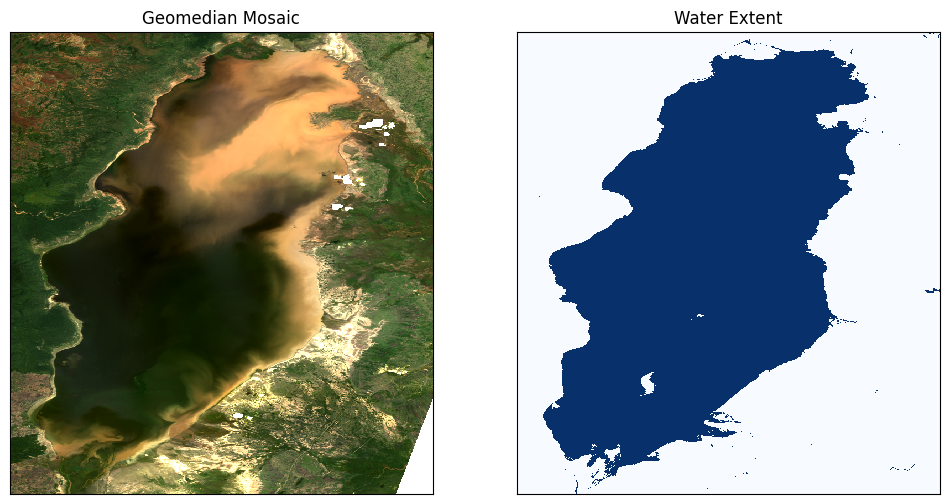
Si les paramètres par défaut étaient utilisés, nous devrions voir que le lac Manyara semble être considérablement pollué dans la moitié nord le 16 février 2016.

Algorithmes de mesure des sédiments en suspension

Nous allons d’abord calculer la qualité de l’eau en utilisant chacun des algorithmes, puis nous comparerons les approches.

(1) Matières en suspension totales (MST) Lymburner

Article : Lymburner et al. 2016 <https://www.sciencedirect.com/science/article/abs/pii/S0034425716301560>

Unités de concentration en mg/L

TSM pour Landsat 7 :

\[LYM7 = 3983 \cdot (\frac{(\text{Vert} + \text{Rouge}) * 0,0001}{2})^{1,6246}\]

TSM pour Landsat 8 :

\[LYM8 = 3957 \cdot (\frac{(\text{Vert} + \text{Rouge}) * 0,0001}{2})^{1,6436}\]

Ici, nous utilisons Landsat 8, nous utiliserons donc la fonction LYM8.

# Function to calculate Lymburner TSM value for Landsat 7
def LYM7(dataset):
    return 3983 * ((dataset.green + dataset.red) * 0.0001 / 2) ** 1.6246

# Function to calculate Lymburner TSM value for Landsat 8
def LYM8(dataset):
    return 3957 * ((dataset.green + dataset.red) * 0.0001 / 2) ** 1.6436

# Calculate the Lymburner TSM value for Landsat 8, using water extent to mask
lym8 = LYM8(ds).where(water_extent)

# Determine the 2% and 98% quantiles and set as min and max respectively
lym8_min = lym8.quantile(0.02).values
lym8_max = lym8.quantile(0.98).values

(2) Modèle de particules en suspension (SPM)

Article : Zhongfeng Qiu et.al. 2013

Unités de concentration en g/m³

SPM pour Landsat 8 :

\[X = 2,26*(\frac{\text{Rouge}}{\text{Vert}})^3 - 5,42*(\frac{\text{Rouge}}{\text{Vert}})^2 + 5,58*(\frac{\text{Rouge}}{\text{Vert}}) - 0,72\]

\[SPM = 10^{X} - 1,43\]

# Function to calculate Suspended Particulate Model value
def SPM_QIU(dataset):
    return (
        10 ** (
            2.26 * (dataset.red / dataset.green) ** 3
            - 5.42 * (dataset.red / dataset.green) ** 2
            + 5.58 * (dataset.red / dataset.green)
            - 0.72
        )
        - 1.43
    )

# Calculate the SPM value for Landsat 8, using water extent to mask
spm_qiu = SPM_QIU(ds).where(water_extent)

# Determine the 2% and 98% quantiles and set as min and max respectively
spm_qiu_min = spm_qiu.quantile(0.02).values
spm_qiu_max = spm_qiu.quantile(0.98).values

(3) Indice de sédiments en suspension par différence normalisée (NDSSI)

Article : Hossain et al. 2010

NDSSI pour Landsat 7 et 8 :

\[NDSSI = \frac{\text{Bleu}-\text{NIR}}{\text{Bleu}+\text{NIR}}\]

La valeur NDSSI varie de -1 à +1. Les valeurs proches de +1 indiquent une concentration plus élevée de sédiments.

# Function to calculate SNDSSI value
def NDSSI(dataset):
    return (dataset.blue - dataset.nir) / (dataset.blue + dataset.nir)

# Calculate the NDSSI value for Landsat 8, using water extent to mask
ndssi = NDSSI(ds).where(water_extent)

# Determine the 2% and 98% quantiles and set as min and max respectively
ndssi_min = ndssi.quantile(0.02).compute().values
ndssi_max = ndssi.quantile(0.98).compute().values

(4) Matières solides totales en suspension (TSS) de Quang

Article : Quang et al. 2017

Unités de concentration en mg/L

\[Quang8 = 380,32 * \text{Rouge}*0,0001 - 1,7826\]

# Function to calculate quang8 value
def QUANG8(dataset):
    return 380.32 * (dataset.red) * 0.0001 - 1.7826

# Calculate the quang8 value for Landsat 8, using water extent to mask
quang8 = QUANG8(ds).where(water_extent)

# Determine the 2% and 98% quantiles and set as min and max respectively
quang8_min = quang8.quantile(0.02).compute().values
quang8_max = quang8.quantile(0.98).compute().values

Comparer les résultats des algorithmes

fig, ax = plt.subplots(2, 2, figsize=(12, 12))
cmap='magma'

lym8.plot(
    ax=ax[0, 0], cmap=cmap, add_colorbar=False, vmin=lym8_min, vmax=lym8_max
)

spm_qiu.plot(
    ax=ax[0, 1], cmap=cmap, add_colorbar=False, vmin=spm_qiu_min, vmax=spm_qiu_max
)

ndssi.plot(
    ax=ax[1, 0], cmap=cmap, add_colorbar=False, vmin=ndssi_min, vmax=ndssi_max
)

quang8.plot(
    ax=ax[1, 1], cmap=cmap, add_colorbar=False, vmin=quang8_min, vmax=quang8_max
)

print(
    "Total Suspended Matter (Black=Low, Purple=Medium-Low, "
    "Orange=Medium-High, Yellow=High)"
)

# Titles
ax[0, 0].set_title("TSM = Leo Lymburner"), ax[0, 0].xaxis.set_visible(False), ax[0, 0].yaxis.set_visible(False)
ax[0, 1].set_title("TSM = Zhongfeng Qui"), ax[0, 1].xaxis.set_visible(False), ax[0, 1].yaxis.set_visible(False)
ax[1, 0].set_title("TSM = NDSSI (Hossain)"), ax[1, 0].xaxis.set_visible(False), ax[1, 0].yaxis.set_visible(False)
ax[1, 1].set_title("TSM = Quang Pham"), ax[1, 1].xaxis.set_visible(False), ax[1, 1].yaxis.set_visible(False)

plt.tight_layout();

Total Suspended Matter (Black=Low, Purple=Medium-Low, Orange=Medium-High, Yellow=High)

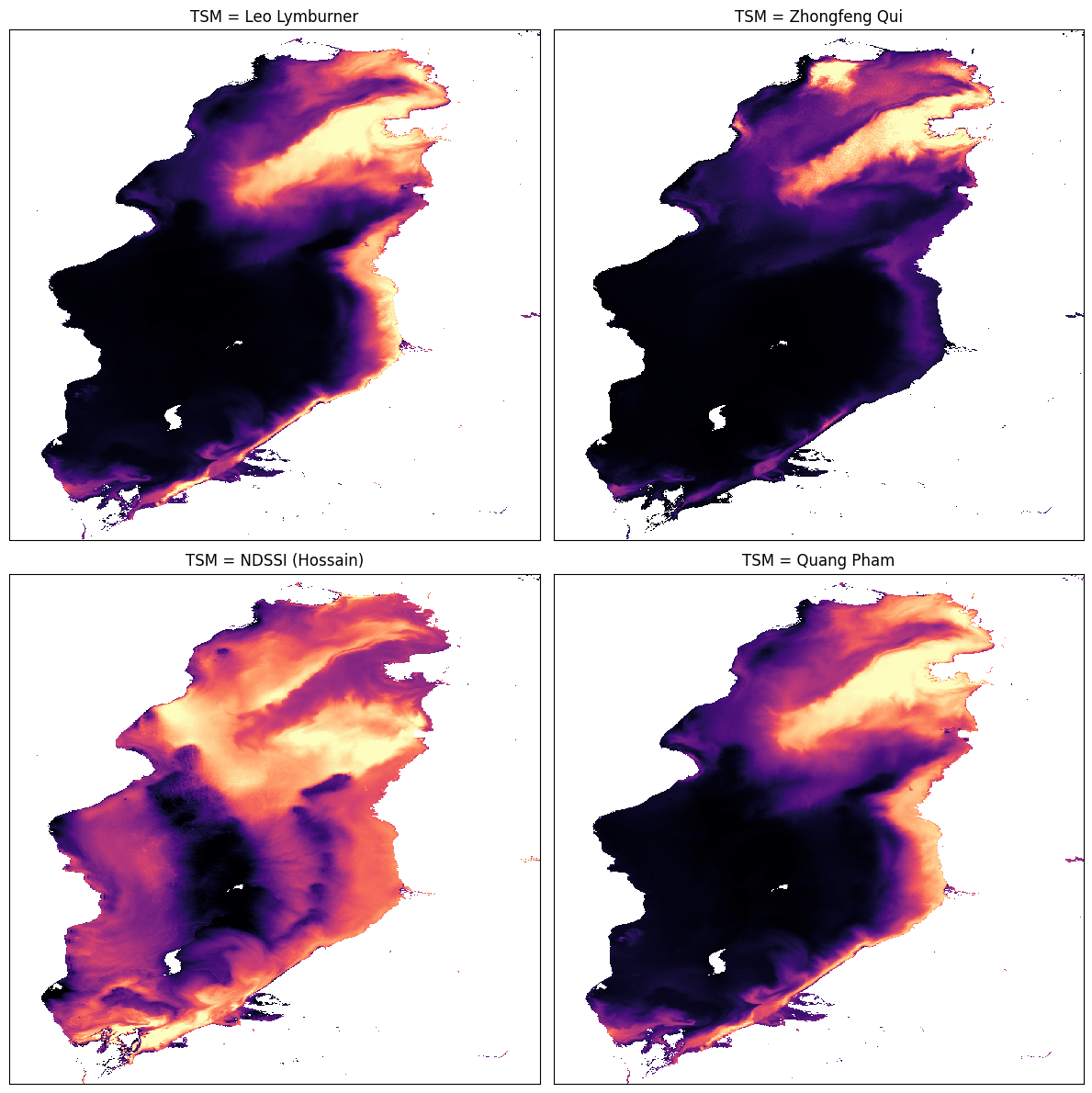
Si les paramètres par défaut étaient utilisés, nous devrions voir que tous les indices reflètent l’apparence du lac (là où il est trouble, l’indice est élevé) à l’exception du NDSSI, bien qu’il semble être lié aux autres - principalement faible là où les autres sont élevés et vice versa.

---

Informations Complémentaires

Licence Le code de ce notebook est sous licence Apache, version 2.0 <https://www.apache.org/licenses/LICENSE-2.0>`__.

Les données de Digital Earth Africa sont sous licence Creative Commons Attribution 4.0 <https://creativecommons.org/licenses/by/4.0/>.

Contact Si vous avez besoin d’aide, veuillez poster une question sur le canal Slack DE Africa <https://digitalearthafrica.slack.com/> ou sur le GIS Stack Exchange <https://gis.stackexchange.com/questions/ask?tags=open-data-cube> en utilisant la balise open-data-cube (vous pouvez consulter les questions posées précédemment `ici <https://gis.stackexchange.com/questions/tagged/open-data-

Si vous souhaitez signaler un problème avec ce notebook, vous pouvez en déposer un sur Github.

Version de Datacube compatible

print(datacube.__version__)

1.8.20

Dernier test :

from datetime import datetime
datetime.today().strftime('%Y-%m-%d')

'2025-01-16'