Identification des navires avec Sentinel-1
Produits utilisés : s1_rtc wofs_ls_summary_annual
Aperçu
La capacité à repérer les navires et les voies de navigation à partir d’images satellite peut être utile pour obtenir une image globale du trafic maritime. Les propriétés des données radar peuvent être utilisées pour détecter où les navires apparaissent au fil du temps, ainsi que pour mettre en évidence la présence de voies de navigation.
Lorsque l’on travaille avec des données radar, l’eau apparaît généralement sombre en raison de sa surface relativement lisse, ce qui entraîne une très faible rétrodiffusion et, par conséquent, de faibles intensités sont enregistrées par le satellite dans les deux bandes de polarisation. Cependant, si un grand navire se trouve sur l’eau, la rétrodiffusion à l’emplacement du navire sera beaucoup plus élevée que celle de l’eau en raison des effets de diffusion à double rebond.
La mission Sentinel-1 de l’ESA/CE Copernicus (Sentinel-1A et 1B) est soumise à une fréquence de revisite de quelques jours. Cela permet de constituer un vaste catalogue d’observations qui peuvent être exploitées pour identifier les voies de navigation.
Dans cet exemple, nous tentons d’identifier les navires autour du canal de Suez en Égypte en mars 2021. Des changements significatifs dans le nombre et le schéma de répartition des navires sont détectés, montrant l’impact d’un blocage. Vous trouverez plus d’informations sur l’événement dans ce fil sur Twitter.
Description
Les navires sont identifiés en tirant parti du fait que les navires sur l’eau génèrent un signal de rétrodiffusion radar important.
Les étapes démontrées dans ce cahier incluent :
Chargement de l’image de rétrodiffusion Sentinel-1 pour une zone d’intérêt.
Extraction du masque d’eau libre à l’aide du résumé annuel des observations de l’eau depuis l’espace (WOfS).
Compter le nombre de navires avant et après l’événement et enregistrer les résultats.
Visualisez les valeurs maximales de rétrodiffusion d’une série chronologique pour identifier les voies de navigation.
Commencer
Pour exécuter cette analyse, exécutez toutes les cellules du bloc-notes, en commençant par la cellule « Charger les packages ».
Charger des paquets
Importez les packages Python utilisés pour l’analyse.
[1]:
%matplotlib inline

import xarray as xr
import numpy as np
import geopandas as gpd
import matplotlib.pyplot as plt

import datacube
from odc.geo.geom import Geometry
from deafrica_tools.spatial import xr_vectorize, xr_rasterize
from deafrica_tools.plotting import display_map
from deafrica_tools.datahandling import load_ard, wofs_fuser, dilate
from deafrica_tools.areaofinterest import define_area
Se connecter au datacube
Connectez-vous au datacube pour que nous puissions accéder aux données de DE Africa. Le paramètre « app » est un nom unique pour l’analyse qui est basé sur le nom du fichier du notebook.
[2]:
dc = datacube.Datacube(app="Ship_detection")
Paramètres d’analyse
La cellule suivante définit les paramètres qui définissent la zone d’intérêt et la durée de l’analyse. Les paramètres sont
« lat » : la latitude centrale à analyser (par exemple « 10,338 »).
« lon » : la longitude centrale à analyser (par exemple « -1,055 »).
« buffer » : le nombre de degrés carrés à charger autour de la latitude et de la longitude centrales. Pour des temps de chargement raisonnables, définissez cette valeur sur « 0,1 » ou moins.
time_range: la plage de dates à analyser (par exemple('2021'))
Sélectionnez l’emplacement
Pour définir la zone d’intérêt, deux méthodes sont disponibles :
En spécifiant la latitude, la longitude et la zone tampon. Cette méthode nécessite que vous saisissiez la latitude centrale, la longitude centrale et la valeur de la zone tampon en degrés carrés autour du point central que vous souhaitez analyser. Par exemple, « lat = 10,338 », « lon = -1,055 » et « buffer = 0,1 » sélectionneront une zone avec un rayon de 0,1 degré carré autour du point avec les coordonnées (10,338, -1,055).
Vous pouvez également fournir des valeurs de tampon distinctes pour la latitude et la longitude d’une zone rectangulaire. Par exemple, « lat = 10.338 », « lon = -1.055 » et « lat_buffer = 0.1 » et « lon_buffer = 0.08 » sélectionneront une zone rectangulaire s’étendant sur 0,1 degré au nord et au sud et 0,08 degré à l’est et à l’ouest à partir du point « (10.338, -1.055) ».
Pour des temps de chargement raisonnables, définissez la mémoire tampon sur « 0,1 » ou moins.
By uploading a polygon as a
GeoJSON or Esri Shapefile. If you choose this option, you will need to upload the geojson or ESRI shapefile into the Sandbox using Upload Files button in the top left corner of the Jupyter Notebook interface. ESRI shapefiles must be uploaded with all the related files
 (.cpg, .dbf, .shp, .shx). Once uploaded, you can use the shapefile or geojson to define the area of interest. Remember to update the code to call the file you have uploaded.
Pour utiliser l’une de ces méthodes, vous pouvez décommenter la ligne de code concernée et commenter l’autre. Pour commenter une ligne, ajoutez le symbole "#" avant le code que vous souhaitez commenter. Par défaut, la première option qui définit l’emplacement à l’aide de la latitude, de la longitude et du tampon est utilisée.
Si vous exécutez le bloc-notes pour la première fois, conservez les paramètres par défaut ci-dessous. Cela montrera comment fonctionne l’analyse et fournira des résultats significatifs. L’exemple porte sur le canal de Suez en Égypte en mars 2021.
[3]:
# Method 1: Specify the latitude, longitude, and buffer
aoi = define_area(lat=29.95, lon=32.536, buffer=0.1)

# Method 2: Use a polygon as a GeoJSON or Esri Shapefile.
# aoi = define_area(vector_path='aoi.shp')

#Create a geopolygon and geodataframe of the area of interest
geopolygon = Geometry(aoi["features"][0]["geometry"], crs="epsg:4326")
geopolygon_gdf = gpd.GeoDataFrame(geometry=[geopolygon], crs=geopolygon.crs)

# Get the latitude and longitude range of the geopolygon
lat_range = (geopolygon_gdf.total_bounds[1], geopolygon_gdf.total_bounds[3])
lon_range = (geopolygon_gdf.total_bounds[0], geopolygon_gdf.total_bounds[2])


# timeframe
timerange = ('2021-03-21', '2021-03-25')
Afficher l’emplacement sélectionné
La cellule suivante affichera la zone sélectionnée sur une carte interactive. N’hésitez pas à zoomer et dézoomer pour mieux comprendre la zone que vous allez analyser. En cliquant sur n’importe quel point de la carte, vous découvrirez les coordonnées de latitude et de longitude de ce point.
[4]:
display_map(x=lon_range, y=lat_range)
[4]:
Charger et afficher les données Sentinel-1
La première étape de l’analyse consiste à charger les données de rétrodiffusion Sentinel-1 pour la zone d’intérêt spécifiée.
[5]:
# Load the Sentinel-1 data
S1 = load_ard(dc=dc,
              products=["s1_rtc"],
              measurements=['vv', 'vh'],
              y=lat_range,
              x=lon_range,
              time=timerange,
              group_by="solar_day"
              )
print(S1)
Using pixel quality parameters for Sentinel 1
Finding datasets
    s1_rtc
Applying pixel quality/cloud mask
Loading 3 time steps
<xarray.Dataset> Size: 24MB
Dimensions:      (time: 3, latitude: 1000, longitude: 1000)
Coordinates:
  * time         (time) datetime64[ns] 24B 2021-03-21T03:44:49.596587 ... 202...
  * latitude     (latitude) float64 8kB 30.05 30.05 30.05 ... 29.85 29.85 29.85
  * longitude    (longitude) float64 8kB 32.44 32.44 32.44 ... 32.64 32.64 32.64
    spatial_ref  int32 4B 4326
Data variables:
    vv           (time, latitude, longitude) float32 12MB 0.04583 ... 0.1556
    vh           (time, latitude, longitude) float32 12MB 0.009784 ... 0.004633
Attributes:
    crs:           EPSG:4326
    grid_mapping:  spatial_ref
/opt/venv/lib/python3.12/site-packages/dask/array/reductions.py:654: RuntimeWarning: All-NaN slice encountered
  return np.nanmax(x_chunk, axis=axis, keepdims=keepdims)
Filtrage des taches en option
Le filtrage Specke n’est pas appliqué dans cet exemple car il existe un contraste élevé entre les signaux de l’eau et ceux du navire. L’application d’un filtrage Specke avec une petite fenêtre de lissage peut aider à améliorer la sensibilité des petits navires.
Un exemple d’application d’un filtre moucheté peut être trouvé dans le « carnet de détection d’eau par radar <Radar_water_detection.ipynb> »__.
Convertir les données en décibels (dB)
Les données de rétrodiffusion de Sentinel-1 comportent deux mesures, VV et VH, qui correspondent à la polarisation de la lumière envoyée et reçue par le satellite. VV fait référence au satellite qui envoie de la lumière polarisée verticalement et reçoit en retour de la lumière polarisée verticalement, tandis que VH fait référence au satellite qui envoie de la lumière polarisée verticalement et reçoit en retour de la lumière polarisée horizontalement. Ces deux bandes de mesure peuvent nous fournir des informations différentes sur la zone que nous étudions.
Lorsque l’on travaille avec la rétrodiffusion radar, il est courant de travailler avec les données en unités de décibels (dB), plutôt qu’en intensité linéaire. Pour convertir le nombre numérique (DN) enregistré en dB dans l’imagerie Sentinel-1, nous utilisons la formule suivante :
[6]:
# Scale to plot data in decibels
S1["vh_dB"] = 10 * np.log10(S1.vh)
S1["vv_dB"] = 10 * np.log10(S1.vv)
/opt/venv/lib/python3.12/site-packages/xarray/core/computation.py:824: RuntimeWarning: divide by zero encountered in log10
  result_data = func(*input_data)
Visualiser les données avant et après l’événement
Nous nous concentrons sur les premières et dernières observations de cette période. L’incident de blocage du navire a commencé le 23 mars 2021 et a duré près d’une semaine. Nous examinons donc une image d’avant l’événement et une autre pendant.
Les images ci-dessous montrent un contraste élevé entre la surface sombre de l’eau et les navires lumineux.
[7]:
fig, (ax1, ax2) = plt.subplots(nrows=1, ncols=2, figsize=(18, 7))

# Visualise baseline image before the event
S1.vv_dB.isel(time=0).plot(robust=True, ax=ax1)

# Visualise the image after the event
S1.vv_dB.isel(time=2).plot(robust=True, ax=ax2);

Extraire la zone d’eau libre
Les eaux de surface peuvent être cartographiées en définissant un seuil de rétrodiffusion radar. Un exemple détaillé est fourni dans le carnet de détection d’eau radar <Radar_water_detection.ipynb>. Pour éliminer l’impact des navires et des vagues, qui provoquent tous deux une rétrodiffusion élevée, des valeurs de rétrodiffusion minimales détectées au fil du temps pour chaque pixel peuvent être utilisées. p.ex.
water_mask = S1.vv.min(dim="time")<0.015
Pour ce carnet, nous utilisons cependant un autre produit facilement disponible en Afrique de l’Ouest, à savoir le résumé annuel des observations de l’eau depuis l’espace (WOfS) pour extraire la zone d’eau libre.
La mesure de « fréquence » de détection d’eau du résumé annuel WOfS de la dernière année disponible est chargée pour correspondre à la grille de pixels Sentinel-1 à l’aide de l’option « like » dans « dc.load() » et du rééchantillonnage « bilinéaire ».
[8]:
# Load WOfS summary through the datacube
wofs = dc.load(product='wofs_ls_summary_annual',
               measurements=['frequency'],
               like=S1.geobox,
               resampling='bilinear',
               time='2019',
               )
La surface d’eau libre est extraite là où l’eau a été détectée plus de 80 % de l’année. Pour un résultat optimal, le masque est encore ajusté pour éliminer les interstices et les petits plans d’eau.
[9]:
# Select pixels that are classified as water > 80 % of the year
water_mask = wofs.frequency > 0.8
[10]:
water_mask.plot(size=6);

[11]:
# close small holes within the water mask and remove a few pixels on the edge for cleaner result
water_mask = xr.DataArray(dilate(~dilate(water_mask, 3, invert=False), 5, invert=True),
                          dims=water_mask.dims).assign_coords(water_mask.coords)
[12]:
# optional step to select only the largest water body

water_bodies = xr_vectorize(water_mask,
                            crs=S1.crs,  # wofs crs is not recoganized, so using S1 instead as they are the same
                            mask=water_mask.values == 1)

largest = water_bodies[water_bodies.area == water_bodies.area.max()]

# create mask
water_mask = xr_rasterize(largest, S1, crs = S1.crs)
/tmp/ipykernel_8214/1524444574.py:7: UserWarning: Geometry is in a geographic CRS. Results from 'area' are likely incorrect. Use 'GeoSeries.to_crs()' to re-project geometries to a projected CRS before this operation.

  largest = water_bodies[water_bodies.area == water_bodies.area.max()]
[13]:
# final water mask
water_mask.plot();

Appliquer un masque d’eau et un seuil pour la détection des navires
Dans cet exemple, un seuil de 0 dB est choisi. Les navires sont détectés lorsque les valeurs de rétrodiffusion sont supérieures à ce seuil. L’image binaire est vectorisée afin que les pixels d’un même navire soient regroupés en un seul objet.
L’inspection visuelle confirme la détection raisonnable des grands cargos. Le seuil peut être ajusté en fonction des différentes zones et des différents types de navires. Avec des emplacements de navires connus, le seuil peut être optimisé à l’aide de données d’apprentissage.
[14]:
# set ship detection threshold in vv to 0 dB
ship_vv_db = 0
[15]:
def detect_ships(da, time_idx, thresh, crs=S1.crs):
    # Thresholding to detect ships
    S1_ships = da.isel(time=time_idx) > thresh

    # Check if S1_ships coordinates match water_mask coordinates
    if not (S1_ships.latitude.equals(water_mask.latitude) and S1_ships.longitude.equals(water_mask.longitude)):
        # Convert boolean array to numeric (0 or 1)
        S1_ships_numeric = S1_ships.astype(int)

        # Align S1_ships with water_mask's longitude and latitude coordinates
        S1_ships = S1_ships_numeric.interp(latitude=water_mask.latitude,
                                           longitude=water_mask.longitude,
                                           method='nearest')

    S1_ships = S1_ships.where(water_mask.values == 1)

    # Vectorize ships
    ships_vector = xr_vectorize(S1_ships,
                                crs=crs,
                                mask=S1_ships.values == 1)

    return ships_vector
[16]:
time_idx = 0
ships_time0 = detect_ships(S1.vv_dB, time_idx, ship_vv_db)
ships_time0.to_file(
f'ships_{str(S1.time.values[time_idx])[0:10]}.geojson', driver='GeoJSON')
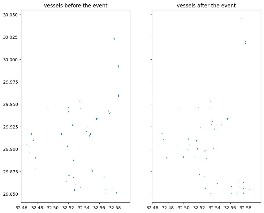
print("Number of ships detected at this time:", len(ships_time0))
Number of ships detected at this time: 51
[17]:
time_idx = 2
ships_time2 = detect_ships(S1.vv_dB, time_idx, ship_vv_db)
ships_time2.to_file(
    f'ships_{str(S1.time.values[time_idx])[0:10]}.geojson', driver='GeoJSON')
print("Number of ships detected at this time:", len(ships_time2))
Number of ships detected at this time: 69
[18]:
# visualize the ship locations

fig, ax = plt.subplots(1, 2, figsize=(10, 10), sharex=True, sharey=True)
ships_time0.plot(ax=ax[0])
ships_time2.plot(ax=ax[1])
ax[0].set_title('vessels before the event')
ax[1].set_title('vessels after the event');
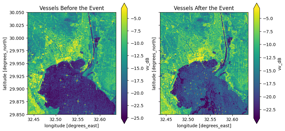
[19]:
# visualize the ship locations over image

fig, ax = plt.subplots(1, 2, figsize=(10, 5), sharex=True, sharey=True)

# Visualize vv_dB underneath ships for the first time index
S1.vv_dB.isel(time=0).plot(robust=True, ax=ax[0])
ships_time0.plot(ax=ax[0], color='red', markersize=50)
ax[0].set_title('Vessels Before the Event')

# Visualize vv_dB underneath ships for the third time index
S1.vv_dB.isel(time=2).plot(robust=True, ax=ax[1])
ships_time2.plot(ax=ax[1], color='red', markersize=50)
ax[1].set_title('Vessels After the Event')

plt.show()
Mises en garde et améliorations possibles
Nous avons appliqué une méthode de seuillage simple pour identifier les navires dans les sections ci-dessus. Seule la rétrodiffusion VV a été utilisée et aucun filtrage de speckle n’a été effectué. Cette méthode est basée sur l’hypothèse que les navires produisent des signaux de rétrodiffusion très élevés et que tous les objets brillants dans la zone d’eau sont des navires.
Des analyses complémentaires peuvent aider à améliorer la méthode :
Le seuil des pixels des navires est choisi en fonction d’une évaluation visuelle. Le seuil est relativement élevé, de sorte que les navires plus petits peuvent être manqués. Ce seuil peut être optimisé avec des données d’entraînement étiquetées pour des cas d’utilisation spécifiques.
Il n’est pas certain que tous les objets brillants à proximité des quais soient des navires. L’emplacement et la forme des objets peuvent être utilisés pour éliminer les faux positifs.
Les structures rigides à bord des navires peuvent entraîner la formation de plusieurs points lumineux déconnectés au-dessus d’un navire. Ces objets plus petits peuvent être regroupés pour obtenir un décompte plus fiable des navires.
Malgré les limitations ci-dessus, nous démontrons qu’avec quelques étapes d’analyse, la rétrodiffusion Sentinel-1 de DE Africa peut être utilisée pour détecter et compter les gros navires.
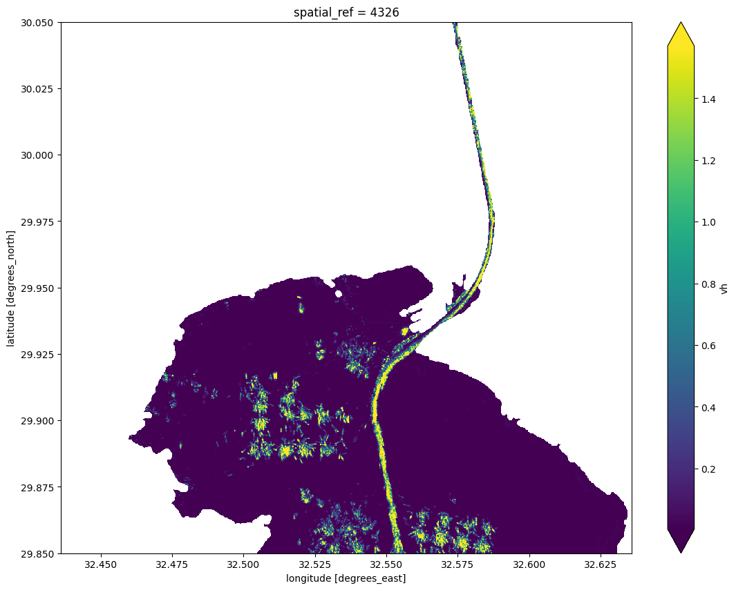
Identifier les voies de navigation
Les emplacements des navires détectés au fil du temps peuvent être utilisés pour cartographier les itinéraires populaires.
Dans les cellules ci-dessous, nous chargeons toutes les observations Sentinel-1 de 2020. Le traçage des valeurs maximales de rétrodiffusion au fil du temps permet une identification claire des voies de navigation.
Les données sont chargées de manière différée à l’aide des options « dask_chunks » pour réduire les besoins en mémoire.
[20]:
# Load the Sentinel-1 data
S1 = load_ard(dc=dc,
              products=["s1_rtc"],
              measurements=['vv', 'vh'],
              y=lat_range,
              x=lon_range,
              time='2020',
              group_by="solar_day",
              dask_chunks={},
              )
Using pixel quality parameters for Sentinel 1
Finding datasets
    s1_rtc
Applying pixel quality/cloud mask
Returning 227 time steps as a dask array
[21]:
# rereate the water mask using the newly loaded S1 to rasterise the largest water body
water_mask = xr_rasterize(largest, S1)

S1.vh.where(water_mask.values == 1).max(dim='time').plot.imshow(robust=True, size=10);
Prochaines étapes
Lorsque vous avez terminé, revenez à la cellule « Configurer l’analyse », modifiez certaines valeurs (par exemple « latitude » et « longitude ») et réexécutez l’analyse.
Plusieurs ports clés sont couverts par les données Sentinel-1 en Afrique. Les données disponibles peuvent être consultées sur le site DEAfrica Explorer <https://explorer.digitalearth.africa/products/s1_rtc>, mais nous listons également les coordonnées de latitude et de longitude de quelques ports clés ci-dessous.
Port de Durban en Afrique du Sud
latitude = -29.87
longitude = 31.03
Port de Dar Es Salaam en Tanzanie
latitude = -6.83
longitude = 39.29
Port de Tanger Med au Maroc
latitude = 35.86
longitude = -5.53
Informations Complémentaires
Licence Le code de ce notebook est sous licence Apache, version 2.0 <https://www.apache.org/licenses/LICENSE-2.0>`__.
Les données de Digital Earth Africa sont sous licence Creative Commons Attribution 4.0 <https://creativecommons.org/licenses/by/4.0/>.
Contact Si vous avez besoin d’aide, veuillez poster une question sur le canal Slack DE Africa <https://digitalearthafrica.slack.com/> ou sur le GIS Stack Exchange <https://gis.stackexchange.com/questions/ask?tags=open-data-cube> en utilisant la balise open-data-cube (vous pouvez consulter les questions posées précédemment `ici <https://gis.stackexchange.com/questions/tagged/open-data-
Si vous souhaitez signaler un problème avec ce notebook, vous pouvez en déposer un sur Github.
Version de Datacube compatible
[22]:
print(datacube.__version__)
1.8.20
Dernier test :
[23]:
from datetime import datetime
datetime.today().strftime('%Y-%m-%d')
[23]:
'2025-01-16'