Prévision de l’état de la végétation des terres cultivées
Mots clés données utilisées ; sentinelle 2, données utilisées ; crop_mask, :index: méthodes de données ; prévision, :index: méthodes de données ; autorégression
Aperçu
Ce carnet de notes effectue des prévisions de séries chronologiques de l’état de la végétation (NDVI) à l’aide de SARIMAX, une variante des modèles « autorégressifs à moyenne mobile (ARMA) <https://en.wikipedia.org/wiki/Autoregressive%E2%80%93moving-average_model#ARMAX> »__ qui comprend un composant intégré (I) pour différencier les séries chronologiques afin qu’elles deviennent stationnaires, un composant saisonnier (S) et a la capacité de prendre en compte les variables exogènes (X).
Dans cet exemple, nous allons réaliser une prévision sur une série temporelle NDVI univariée. Autrement dit, notre prévision sera construite sur des modèles temporels dans le NDVI. À l’inverse, les approches multivariées peuvent tenir compte de l’influence de variables telles que l’humidité du sol et les précipitations.
Description
Dans ce notebook, nous générons une série temporelle NDVI à partir de Sentinel-2, puis l’utilisons pour développer un algorithme de prévision.
Les mesures suivantes sont prises :
Chargez les données Sentinel-2 et calculez le NDVI.
Masquez le NDVI sur les terres cultivées à l’aide du masque de culture.
Parcourez les paramètres SARIMAX et effectuez une sélection de modèle basée sur une validation croisée.
Inspecter les diagnostics du modèle
Prévoyez le NDVI dans le futur et visualisez le résultat.
Charger des paquets
Importez les packages Python utilisés pour l’analyse.
Remarque importante : Scipy a été mis à jour et présente certaines incompatibilités avec les anciennes versions de statsmodels. Si la cellule de chargement des packages ci-dessous renvoie une erreur, essayez d’exécuter « pip install statsmodels » ou « pip install statsmodels –upgrade » dans une cellule de code, puis chargez à nouveau les packages.
[1]:
%matplotlib inline
from itertools import product

import datacube
import numpy as np
import pandas as pd
import geopandas as gpd
import statsmodels.api as sm
import xarray as xr
from datacube import Datacube

from odc.geo.geom import Geometry
from deafrica_tools.spatial import xr_rasterize
from deafrica_tools.bandindices import calculate_indices
from deafrica_tools.dask import create_local_dask_cluster
from deafrica_tools.datahandling import load_ard
from deafrica_tools.plotting import display_map
from matplotlib import pyplot as plt
from statsmodels.tools.eval_measures import rmse
from tqdm.notebook import tqdm
from deafrica_tools.areaofinterest import define_area
Configurer un cluster Dask
Dask peut être utilisé pour mieux gérer l’utilisation de la mémoire et effectuer l’analyse en parallèle. Pour une introduction à l’utilisation de Dask avec Digital Earth Africa, consultez le Dask notebook.
Remarque : nous vous recommandons d’ouvrir la fenêtre de traitement Dask pour afficher les différents calculs en cours d’exécution ; pour ce faire, consultez la section Tableau de bord Dask en Afrique de l’Ouest du Dask notebook.
Pour utiliser Dask, configurez le cluster de calcul local à l’aide de la cellule ci-dessous.
[2]:
create_local_dask_cluster()
/opt/venv/lib/python3.12/site-packages/distributed/node.py:187: UserWarning: Port 8787 is already in use.
Perhaps you already have a cluster running?
Hosting the HTTP server on port 36459 instead
  warnings.warn(
Client
Client-d59ed3b7-d44a-11ef-a9ee-1e01ca941b00
| Connection method: Cluster object | Cluster type: distributed.LocalCluster |
| Dashboard: /user/victoria@kartoza.com/proxy/36459/status |
Cluster Info
LocalCluster
01a14b58
| Dashboard: /user/victoria@kartoza.com/proxy/36459/status | Workers: 1 |
| Total threads: 7 | Total memory: 59.21 GiB |
| Status: running | Using processes: True |
Scheduler Info
Scheduler
Scheduler-931a3ae0-a1cb-4fca-b6ff-760875560357
| Comm: tcp://127.0.0.1:35489 | Workers: 1 |
| Dashboard: /user/victoria@kartoza.com/proxy/36459/status | Total threads: 7 |
| Started: Just now | Total memory: 59.21 GiB |
Workers
Worker: 0
| Comm: tcp://127.0.0.1:44715 | Total threads: 7 |
| Dashboard: /user/victoria@kartoza.com/proxy/38151/status | Memory: 59.21 GiB |
| Nanny: tcp://127.0.0.1:38883 | |
| Local directory: /tmp/dask-scratch-space/worker-twr95w88 | |
Se connecter au datacube
[3]:
dc = datacube.Datacube(app="NDVI_forecast")
Paramètres d’analyse
« lat », « lon » : la latitude et la longitude centrales à analyser. Dans cet exemple, nous utiliserons une zone agricole en Éthiopie.
« buffer » : le nombre de degrés carrés à charger autour de la latitude et de la longitude centrales. Pour des temps de chargement raisonnables, définissez cette valeur sur 0,1 ou moins.
« produits » : les données satellite à charger, dans l’exemple nous utiliserons Sentinel-2.
time_range: la plage de dates à analyser. Plus la plage de dates est longue, plus le modèle dispose de données pour dériver des modèles dans la série chronologique NDVI.freq: La fréquence à laquelle nous voulons rééchantillonner la série chronologique, par exemple pour les pas de temps mensuels, utilisez « 1M », pour les pas de temps bimensuels, utilisez « 2W ».forecast_length: la durée au-delà de la dernière observation dans l’ensemble de données que nous souhaitons que le modèle prévoie, exprimée en unités de fréquence de rééchantillonnage « freq ». Une « forecast_length » plus longue signifie une plus grande incertitude de prévision.« résolution » : la résolution en pixels (en mètres) à utiliser pour le chargement des données Sentinel-2.
« dask_chunks » : Comment fragmenter les ensembles de données pour travailler avec dask.
Sélectionnez l’emplacement
Pour définir la zone d’intérêt, deux méthodes sont disponibles :
En spécifiant la latitude, la longitude et la zone tampon. Cette méthode nécessite que vous saisissiez la latitude centrale, la longitude centrale et la valeur de la zone tampon en degrés carrés autour du point central que vous souhaitez analyser. Par exemple, « lat = 10,338 », « lon = -1,055 » et « buffer = 0,1 » sélectionneront une zone avec un rayon de 0,1 degré carré autour du point avec les coordonnées (10,338, -1,055).
Vous pouvez également fournir des valeurs de tampon distinctes pour la latitude et la longitude d’une zone rectangulaire. Par exemple, « lat = 10.338 », « lon = -1.055 » et « lat_buffer = 0.1 » et « lon_buffer = 0.08 » sélectionneront une zone rectangulaire s’étendant sur 0,1 degré au nord et au sud et 0,08 degré à l’est et à l’ouest à partir du point « (10.338, -1.055) ».
Pour des temps de chargement raisonnables, définissez la mémoire tampon sur « 0,1 » ou moins.
By uploading a polygon as a
GeoJSON or Esri Shapefile. If you choose this option, you will need to upload the geojson or ESRI shapefile into the Sandbox using Upload Files button in the top left corner of the Jupyter Notebook interface. ESRI shapefiles must be uploaded with all the related files
 (.cpg, .dbf, .shp, .shx). Once uploaded, you can use the shapefile or geojson to define the area of interest. Remember to update the code to call the file you have uploaded.
Pour utiliser l’une de ces méthodes, vous pouvez décommenter la ligne de code concernée et commenter l’autre. Pour commenter une ligne, ajoutez le symbole "#" avant le code que vous souhaitez commenter. Par défaut, la première option qui définit l’emplacement à l’aide de la latitude, de la longitude et du tampon est utilisée.
[4]:
# Method 1: Specify the latitude, longitude, and buffer
aoi = define_area(lat=8.5593, lon=40.6975, buffer=0.04)

# Method 2: Use a polygon as a GeoJSON or Esri Shapefile.
#aoi = define_area(vector_path='aoi.shp')

#Create a geopolygon and geodataframe of the area of interest
geopolygon = Geometry(aoi["features"][0]["geometry"], crs="epsg:4326")
geopolygon_gdf = gpd.GeoDataFrame(geometry=[geopolygon], crs=geopolygon.crs)

# Get the latitude and longitude range of the geopolygon
lat_range = (geopolygon_gdf.total_bounds[1], geopolygon_gdf.total_bounds[3])
lon_range = (geopolygon_gdf.total_bounds[0], geopolygon_gdf.total_bounds[2])
[5]:
# the satellite product to load
products = "s2_l2a"

# Define the time window for defining the model
time_range = ("2017-01-01", "2022-01")

# resample frequency
freq = "1ME"

# number of time-steps to forecast (in units of `freq`)
forecast_length = 6

# resolution of Sentinel-2 pixels
resolution = (-20, 20)

# dask chunk sizes
dask_chunks = {"x": 500, "y": 500, "time": -1}
Afficher la zone d’analyse sur une carte interactive
[6]:
display_map(lon_range, lat_range)
[6]:
Charger les données satellite
En utilisant les paramètres que nous avons définis ci-dessus.
[7]:
# set up a datcube query object
query = {
    "x": lon_range,
    "y": lat_range,
    "time": time_range,
    "measurements": ["red", "nir"],
    "output_crs": "EPSG:6933",
    "resolution": resolution,
    "resampling": {"fmask": "nearest", "*": "bilinear"},
}
[8]:
# load the satellite data
ds = load_ard(dc=dc, dask_chunks=dask_chunks, products=products, **query)

print(ds)
Using pixel quality parameters for Sentinel 2
Finding datasets
    s2_l2a
Applying pixel quality/cloud mask
Returning 767 time steps as a dask array
<xarray.Dataset> Size: 1GB
Dimensions:      (time: 767, y: 505, x: 387)
Coordinates:
  * time         (time) datetime64[ns] 6kB 2017-01-06T07:42:19 ... 2022-01-30...
  * y            (y) float64 4kB 1.093e+06 1.093e+06 ... 1.083e+06 1.083e+06
  * x            (x) float64 3kB 3.923e+06 3.923e+06 ... 3.931e+06 3.931e+06
    spatial_ref  int32 4B 6933
Data variables:
    red          (time, y, x) float32 600MB dask.array<chunksize=(767, 500, 387), meta=np.ndarray>
    nir          (time, y, x) float32 600MB dask.array<chunksize=(767, 500, 387), meta=np.ndarray>
Attributes:
    crs:           EPSG:6933
    grid_mapping:  spatial_ref
[9]:
ds
[9]:
<xarray.Dataset> Size: 1GB
Dimensions:      (time: 767, y: 505, x: 387)
Coordinates:
  * time         (time) datetime64[ns] 6kB 2017-01-06T07:42:19 ... 2022-01-30...
  * y            (y) float64 4kB 1.093e+06 1.093e+06 ... 1.083e+06 1.083e+06
  * x            (x) float64 3kB 3.923e+06 3.923e+06 ... 3.931e+06 3.931e+06
    spatial_ref  int32 4B 6933
Data variables:
    red          (time, y, x) float32 600MB dask.array<chunksize=(767, 500, 387), meta=np.ndarray>
    nir          (time, y, x) float32 600MB dask.array<chunksize=(767, 500, 387), meta=np.ndarray>
Attributes:
    crs:           EPSG:6933
grid_mapping: spatial_refMasquer la région avec la carte de l’étendue des terres cultivées de l’Afrique de l’Est
Chargez le masque de culture sur la région d’intérêt. La région par défaut que nous analysons est en Éthiopie, nous devons donc charger soit le produit crop_mask qui couvre l’ensemble du continent africain, soit le produit crop_mask_eastern, qui couvre les pays d’Éthiopie, du Kenya, de Tanzanie, du Rwanda et du Burundi. Si vous modifiez la région d’analyse par défaut, vous devrez peut-être charger un masque de culture différent - consultez la page docs pour en savoir plus.
[10]:
cm = dc.load(
    product="crop_mask",
    time=("2019"),
    measurements="filtered",
    resampling="nearest",
    like=ds.geobox,
).filtered.squeeze()

# convert the missing values (255) to NaN
cm = cm.where(cm != 255)

cm.plot.imshow(add_colorbar=False, figsize=(6, 6))
plt.title("Cropland Extent");
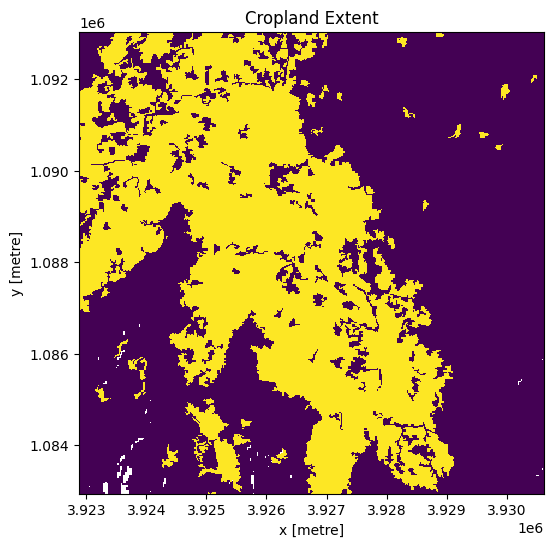
Nous allons maintenant utiliser la carte des terres cultivées pour masquer les régions des données Sentinel-2 qui ne contiennent que des cultures.
[11]:
ds = ds.where(cm == 1)
Découpez les ensembles de données selon la forme de la zone d’intérêt
Un géopolygone représente les limites et non la forme réelle, car il est conçu pour représenter l’étendue de l’entité géographique cartographiée, plutôt que sa forme exacte. En d’autres termes, le géopolygone est utilisé pour définir la limite extérieure de la zone d’intérêt, plutôt que les entités et caractéristiques internes.
Il est important de découper les données selon la forme exacte de la zone d’intérêt, car cela permet de garantir que les données utilisées sont pertinentes pour la zone d’étude spécifique. Bien qu’un géopolygone fournisse des informations sur la limite de l’entité géographique représentée, il ne reflète pas nécessairement la forme ou l’étendue exacte de la zone d’intérêt.
[12]:
#Rasterise the area of interest polygon
aoi_raster = xr_rasterize(gdf=geopolygon_gdf, da=ds, crs=ds.crs)
#Mask the dataset to the rasterised area of interest
ds = ds.where(aoi_raster == 1)
Calculer le NDVI et nettoyer les séries chronologiques
Après avoir calculé le NDVI, nous allons lisser et interpoler les données pour garantir que nous travaillons avec une série chronologique cohérente. Il s’agit d’une étape très importante du flux de travail et il existe de nombreuses façons de lisser, d’interpoler, de combler les lacunes, de supprimer les valeurs aberrantes ou d’ajuster les courbes des données pour garantir une série chronologique cohérente. Si vous n’utilisez pas l’exemple par défaut, vous devrez peut-être définir des méthodes supplémentaires à celles utilisées ici.
Pour ce faire, nous procédons en deux étapes :
Rééchantillonner les données à des intervalles de temps mensuels en utilisant la moyenne
Calculer une moyenne mobile avec une fenêtre de 4 étapes
[13]:
# calculate NDVI
ndvi = calculate_indices(ds, "NDVI", drop=True, satellite_mission="s2")
Dropping bands ['red', 'nir']
[14]:
# resample and smooth
window = 4

ndvi = (
    ndvi.resample(time=freq)
    .mean()
    .rolling(time=window, min_periods=1, center=True)
    .mean()
)
Réduire la série chronologique à une dimension
Dans cet exemple, nous générons une prévision sur une série temporelle 1D simple. Cette série temporelle représente le NDVI moyenné spatialement à chaque pas de temps de la série.
Dans cette étape, tous les calculs ci-dessus sont déclenchés et l’ensemble de données est mis en mémoire. Cette étape peut donc prendre quelques minutes.
[15]:
ndvi = ndvi.mean(["x", "y"])
ndvi = ndvi.NDVI.compute()
/opt/venv/lib/python3.12/site-packages/rasterio/warp.py:387: NotGeoreferencedWarning: Dataset has no geotransform, gcps, or rpcs. The identity matrix will be returned.
  dest = _reproject(
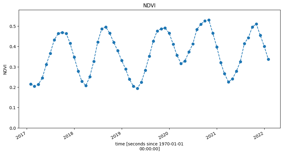
Tracer la série chronologique NDVI
[16]:
ndvi.plot(figsize=(11, 5), linestyle="dashed", marker="o")
plt.title("NDVI")
plt.ylim(0, ndvi.max().values + 0.05);
Diviser les données et ajuster un modèle
La validation croisée est une méthode courante pour évaluer les performances d’un modèle. Elle consiste à diviser les données en un ensemble d’apprentissage sur lequel le modèle est formé et en un ensemble de test (ou de validation) auquel le modèle est appliqué pour produire des prédictions qui sont comparées aux valeurs réelles (qui n’ont pas été utilisées lors de l’apprentissage du modèle).
[17]:
ndvi = ndvi.drop_vars("spatial_ref").to_dataframe()
train_data = ndvi["NDVI"][
    : len(ndvi) - 10
]  # remove the last ten observations and keep them as test data
test_data = ndvi["NDVI"][len(ndvi) - 10 :]
Trouver de manière itérative les meilleurs paramètres pour le modèle SARIMAX
Les modèles SARIMAX sont équipés de paramètres pour les composantes de tendance et saisonnières des séries chronologiques. Les paramètres peuvent être définis comme suit :
Éléments de tendance
p : ordre d’autorégression. Il s’agit du nombre de valeurs immédiatement précédentes dans la série qui sont utilisées pour prédire la valeur à l’instant présent.
d : ordre de différence. Le nombre de fois que la différenciation est effectuée est appelé ordre de différence.
q : Ordre de moyenne mobile. La taille de la fenêtre de moyenne mobile.
Les éléments saisonniers sont les mêmes que ci-dessus, mais pour la composante saisonnière de la série chronologique.
P
D
Q
Nous devons également définir la durée de la saison.
s : Dans ce cas, nous utilisons 6, qui est en unités de fréquence de rééchantillonnage et fait donc référence à 6 mois.
Dans la cellule ci-dessous, les valeurs initiales et une plage sont données pour les paramètres ci-dessus. L’utilisation de range(0, 3) signifie que les valeurs 0, 1 et 2 sont parcourues pour chacun des p, d, q et P, D, Q. Cela signifie qu’il existe \(3^2 \times 3^2 = 81\) combinaisons possibles.
[18]:
# Set initial values and some bounds
p = range(0, 3)
d = 1
q = range(0, 3)
P = range(0, 3)
D = 1
Q = range(0, 3)
s = 6

# Create a list with all possible combinations of parameters
parameters = product(p, q, P, Q)
parameters_list = list(parameters)
print("Number of iterations to run:", len(parameters_list))

# Train many SARIMA models to find the best set of parameters
def optimize_SARIMA(parameters_list, d, D, s):
    """
    Return an ordered (ascending RMSE) dataframe with parameters,
    corresponding AIC, and RMSE.

    parameters_list - list with (p, q, P, Q) tuples
    d - integration order
    D - seasonal integration order
    s - length of season
    """

    results = []
    best_aic = float("inf")

    for param in tqdm(parameters_list):
        try:
            import warnings

            warnings.filterwarnings("ignore")
            model = sm.tsa.statespace.SARIMAX(
                train_data,
                order=(param[0], d, param[1]),
                seasonal_order=(param[2], D, param[3], s),
            ).fit(disp=-1)

            pred = model.predict(start=len(train_data), end=(len(ndvi) - 1))
            error = rmse(pred, test_data)

        except:
            continue

        aic = model.aic

        # Save best model, AIC and parameters
        if aic < best_aic:
            best_model = model
            best_aic = aic
            best_param = param
        results.append([param, model.aic, error])

    result_table = pd.DataFrame(results)
    result_table.columns = ["parameters", "aic", "error"]
    # Sort in ascending order, lower AIC is better
    result_table = result_table.sort_values(by="error", ascending=True).reset_index(
        drop=True
    )

    return result_table
Number of iterations to run: 81
Nous allons maintenant exécuter la fonction ci-dessus pour chaque itération des paramètres que nous avons définis. Selon le nombre d’itérations, l’exécution peut prendre quelques minutes. Une barre de progression est imprimée ci-dessous.
[19]:
# run the function above
result_table = optimize_SARIMA(parameters_list, d, D, s)
Sélection du modèle
L’erreur quadratique moyenne (RMSE) est une mesure courante utilisée pour évaluer les performances d’un modèle ou d’une prévision. Il s’agit de l’écart type des résidus (différence entre la valeur prévue et la valeur réelle) exprimé en unités de la variable d’intérêt, par exemple NDVI. Nous pouvons calculer l’erreur quadratique moyenne de notre prévision car nous avons retenu certaines observations comme données de test ou de validation.
Nous pouvons également utiliser le critère d’information d’Akaike (AIC) <https://en.wikipedia.org/wiki/Akaike_information_criterion>`__ ou le critère d’information bayésien (BIC) <https://en.wikipedia.org/wiki/Bayesian_information_criterion>`__ pour la sélection du modèle. Ces deux critères visent à optimiser le compromis entre la qualité de l’ajustement et la simplicité du modèle. Nous cherchons à trouver le modèle qui peut expliquer le plus de variation dans la série temporelle avec le moins de complexité, car une complexité supplémentaire peut conduire à un surajustement. Le BIC pénalise davantage les paramètres supplémentaires (plus grande complexité) que l’AIC.
Il existe différentes écoles de pensée sur le critère à utiliser. En règle générale, le BIC doit être utilisé pour l’inférence et l’interprétation tandis que l’AIC doit être utilisé pour la prédiction. Comme notre objectif est la prédiction (prévision), nous pourrions sélectionner le modèle avec l’AIC le plus bas, bien que cette approche soit souvent réservée aux cas où il n’y a pas de données de test disponibles pour la validation croisée.
La cellule ci-dessous présente les 15 meilleurs modèles basés sur l’AIC et le RMSE sur la validation croisée.
[20]:
# Sort table by the lowest AIC (Akaike Information Criteria) where the RMSE is low
result_table = result_table.sort_values("aic").sort_values("error")
print(result_table[0:15])
      parameters         aic     error
0   (0, 0, 2, 2) -165.970990  0.017479
1   (2, 2, 0, 1) -204.185850  0.018467
2   (0, 0, 1, 2) -167.675022  0.018694
3   (0, 0, 2, 1) -161.886928  0.019422
4   (0, 1, 1, 1) -185.405325  0.019897
5   (2, 2, 0, 2) -203.090273  0.020219
6   (0, 1, 2, 1) -184.014951  0.020868
7   (2, 2, 2, 2) -198.923767  0.021366
8   (0, 1, 2, 2) -186.460473  0.021840
9   (0, 1, 1, 2) -187.612900  0.023772
10  (2, 1, 1, 2) -198.057996  0.023991
11  (0, 0, 1, 1) -162.146544  0.024082
12  (1, 2, 1, 1) -188.602968  0.027498
13  (2, 1, 1, 1) -190.683099  0.027887
14  (2, 2, 1, 2) -199.563266  0.030304
Sélectionnez le modèle et prédisez
Dans la cellule ci-dessous, nous allons sélectionner un modèle dans la liste ci-dessus. Dans ce cas, nous avons sélectionné le modèle « 0 » car il a le RMSE le plus bas, mais vous pouvez sélectionner n’importe quel modèle en définissant le numéro d’index dans la cellule ci-dessous à l’aide du paramètre « model_sel_index ».
[21]:
# selected model
model_sel_index = 0

# store parameters from selected model
p, q, P, Q = result_table.iloc[model_sel_index].parameters
print(result_table.iloc[model_sel_index])

# fit the model with the parameters identified above
best_model = sm.tsa.statespace.SARIMAX(
    train_data, order=(p, d, q), seasonal_order=(P, D, Q, s)
).fit(disp=-1)
parameters    (0, 0, 2, 2)
aic             -165.97099
error             0.017479
Name: 0, dtype: object
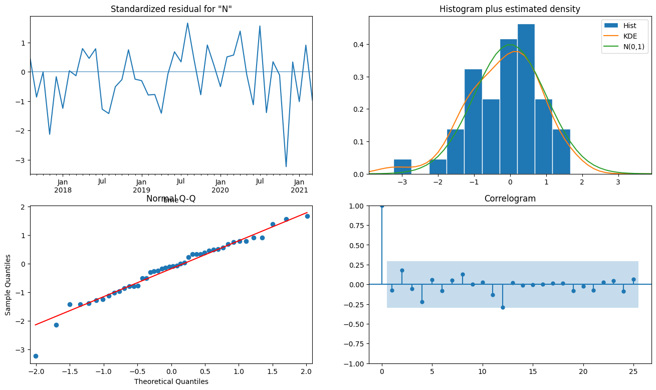
Diagnostic du modèle de tracé
Il existe quelques tracés typiques que nous pouvons utiliser pour évaluer notre modèle.
Résidus normalisés (en haut à gauche) Les résidus normalisés sont représentés en fonction des valeurs x (temps). Cela nous permet de vérifier que la variance (distance des résidus par rapport à 0) est constante au fil du temps. Il ne devrait pas y avoir de tendances évidentes.
Histogramme et densité estimée (en haut à droite) Une estimation de la densité du noyau (KDE) est une fonction de densité de probabilité estimée ajustée sur la distribution réelle (histogramme) des résidus standardisés. Une distribution normale (N (0,1)) est présentée à titre de référence. Ce graphique montre que la distribution de nos résidus standardisés est proche de la distribution normale.
Graphique quantile-quantile normal (Q-Q) (en bas à gauche) Ce graphique montre les quantiles « attendus » ou « théoriques » tirés d’une distribution normale sur l’axe des x par rapport aux quantiles tirés de l’échantillon de résidus sur l’axe des y. Si les observations en bleu correspondent à la ligne 1:1 en rouge, nous pouvons alors conclure que nos résidus sont normalement distribués.
Corrélogramme (en bas à droite) Les corrélations pour les décalages supérieurs à 0 ne devraient pas être statistiquement significatives. Autrement dit, elles ne devraient pas se trouver en dehors du ruban bleu.
Remarque : le graphique Q-Q et le corrélogramme générés pour le modèle « 0 » montrent qu’il existe un certain modèle dans les résidus. En d’autres termes, il existe une variation résiduelle dans les données dont le modèle n’a pas tenu compte. Vous pouvez expérimenter différentes valeurs de paramètres ou différentes sélections de modèles dans les étapes précédentes pour voir si cela peut être résolu.
[22]:
fig = plt.figure(figsize=(16, 9))
fig = best_model.plot_diagnostics(lags=25, fig=fig)
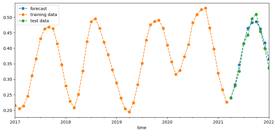
Prévisions de backtest
Nous avons enregistré les 10 dernières observations comme données de test ci-dessus. Nous pouvons maintenant utiliser notre modèle pour prédire le NDVI pour ces intervalles de temps et comparer ces prédictions avec les valeurs réelles. Nous pouvons le faire visuellement dans le graphique ci-dessous et également quantifier l’erreur avec l’erreur quadratique moyenne (RMSE).
[23]:
pred = best_model.predict(start=len(train_data), end=(len(ndvi) - 1))

plt.figure(figsize=(11, 5))
pred.plot(label="forecast", linestyle="dashed", marker="o")
train_data.plot(label="training data", linestyle="dashed", marker="o")
test_data.plot(label="test data", linestyle="dashed", marker="o")
plt.legend(loc="upper left");
Tracez le résultat de notre prévision
Pour prévoir l’indice NDVI dans le futur, nous allons exécuter un modèle sur l’ensemble de la série chronologique afin de pouvoir inclure les dernières observations. Nous pouvons voir que l’incertitude de prévision, exprimée sous la forme d’un intervalle de confiance de 95 %, augmente avec le temps.
[24]:
final_model = sm.tsa.statespace.SARIMAX(
    ndvi, order=(p, d, q), seasonal_order=(P, D, Q, s)
).fit(disp=-1)

yhat = final_model.get_forecast(forecast_length);
[25]:
fig, ax = plt.subplots(1, 1, figsize=(11, 5))
yhat.predicted_mean.plot(label="NDVI forecast", ax=ax, linestyle="dashed", marker="o")
ax.fill_between(
    yhat.predicted_mean.index,
    yhat.conf_int()["lower NDVI"],
    yhat.conf_int()["upper NDVI"],
    alpha=0.2,
)
ndvi[-36:].plot(label="Observaions", ax=ax, linestyle="dashed", marker="o")
plt.legend(loc="upper left");
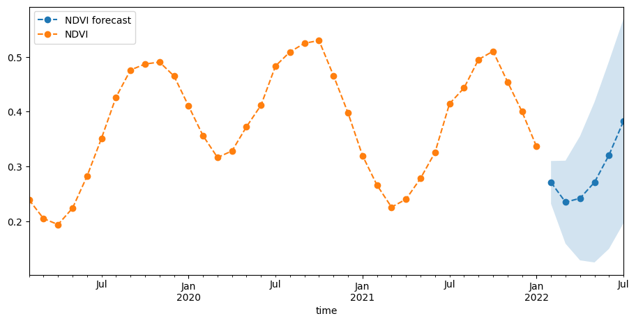
Nos prévisions semblent raisonnables dans le contexte de la série chronologique ci-dessus.
Informations Complémentaires
Licence Le code de ce notebook est sous licence Apache, version 2.0 <https://www.apache.org/licenses/LICENSE-2.0>`__.
Les données de Digital Earth Africa sont sous licence Creative Commons Attribution 4.0 <https://creativecommons.org/licenses/by/4.0/>.
Contact Si vous avez besoin d’aide, veuillez poster une question sur le canal Slack DE Africa <https://digitalearthafrica.slack.com/> ou sur le GIS Stack Exchange <https://gis.stackexchange.com/questions/ask?tags=open-data-cube> en utilisant la balise open-data-cube (vous pouvez consulter les questions posées précédemment `ici <https://gis.stackexchange.com/questions/tagged/open-data-
Si vous souhaitez signaler un problème avec ce notebook, vous pouvez en déposer un sur Github.
Version de Datacube compatible
[26]:
print(datacube.__version__)
1.8.20
Dernier test :
[27]:
from datetime import datetime

datetime.today().strftime("%Y-%m-%d")
[27]:
'2025-01-16'