Inspecting training data

Keywords data methods; principal component analysis, data methods; violin plots, data methods; machine learning, data methods; feature importance

Background

Prior to training a machine learning classifier, it can be useful to understand which of our feature layers are most useful for distinguishing between classes. The feature layers the models are trained on form the knowledge base of the algorithm. We can explore this knowledge base using class-specific violin plots, and through a dimensionality reduction approach called principal component analysis. The latter transforms our large dataset with lots of variables into a smaller dataset with fewer variables (while still preserving much of the variance), this allows us to visualise a very complex dataset in a relatively intuitive and straightforward manner.

By exploring our training data we can learn more about the land cover classes we are interested in mapping (e.g is NDVI a good way to distinguish between crop and non-crop areas?), decide if we have enough training data and the right features for our models to be able to accurately map the classes (are there distinct differences in the feature layers values between classes?), and position ourselves to improve the model should the results be unsatisfactory (what kinds of features can we discard that might be confusing the model?).

Description

Using the training data written to file in the previous notebook, 1_Extract_training_data, this notebook will:

1. Plot class-specific violin plots for each of the feature layers in the training data

2. Plot the importance of each feature after applying a model to the data.

3. Calculate the first two and three prinicpal components of the dataset and plot them as 2D and 3D scatter plots

Getting started

To run this analysis, run all the cells in the notebook, starting with the “Load packages” cell.

Load packages

%matplotlib inline
import random
import numpy as np
import pandas as pd
import seaborn as sns
from pprint import pprint
import matplotlib.pyplot as plt
from matplotlib.patches import Patch
from sklearn.decomposition import PCA
from mpl_toolkits.mplot3d import Axes3D
from sklearn.preprocessing import StandardScaler
from sklearn.ensemble import RandomForestClassifier

Analysis Parameters

• training_data: Name and location of the training data .txt file output from runnning 1_Extract_training_data.ipynb

• class_dict: A dictionary mapping the ‘string’ name of the classes to the integer values that represent our classes in the training data (e.g. {'crop': 1., 'noncrop': 0.})

• field: This is the name of the column in the original training data shapefile that contains the class labels. This is provided simply so we can remove this attribute before we plot the data

training_data = "results/test_training_data.txt"

class_dict = {'crop':1, 'noncrop':0}

field = 'class'

Import training data

# load the data
model_input = np.loadtxt(training_data)

# load the column_names
with open(training_data, 'r') as file:
    header = file.readline()

column_names = header.split()[1:]

# Extract relevant indices from training data
model_col_indices = [column_names.index(var_name) for var_name in column_names[1:]]

Data Wrangling

This cell extracts each class in the training data array and assigns it to a dictionary, this step will allow for cleanly plotting our data

dfs = {}

# Insert data into a Pandas DataFrame, then split into features and labels
model_input_df = pd.DataFrame(model_input, columns=column_names)
X = model_input_df.drop(field, axis=1)
y = model_input_df[[field]]

# Fit the standard scaler to all features
scaler = StandardScaler(with_mean=False)
scaler.fit(X);

for key, value in class_dict.items():
    print(key, value)
    # extract values for class from training data
    arr = model_input[model_input[:,0]==value]
    # create a pandas df for ease of use later
    df = pd.DataFrame(arr).rename(columns={i:column_names[i] for i in range(0,len(column_names))}).drop(field, axis=1)
    # Scale the dataframe
    scaled_df = scaler.transform(df)
    scaled_df = pd.DataFrame(scaled_df, columns=df.columns)

    dfs.update({key:scaled_df})

crop 1
noncrop 0

Feature layer violin plots

#generate a random list of colors same length as num of classes
get_colors = lambda n: list(map(lambda i: "#" + "%06x" % random.randint(0, 0xFFFFFF),range(n)))
colors = get_colors(len(dfs))

#generate list of offsets & widths for plotting
start=-0.2
end=0.2
offsets = list(np.linspace(start,end,len(dfs)))
if len(dfs) == 2:
    width=0.4
else:
    width=np.abs(offsets[0] - offsets[1])

#create figure and axes
fig, ax = plt.subplots(figsize=(40,8))

for key, color, offset in zip(dfs,colors, offsets):
    #create violin plots
    pp = ax.violinplot(dfs[key].values,
                       showmedians=True,
                       positions=np.arange(dfs[key].values.shape[1])+offset, widths=width
                      )
    # change the colour of the plots
    for pc in pp['bodies']:
        pc.set_facecolor(color)
        pc.set_edgecolor(color)
        pc.set_alpha(1)

    #change the line style in the plots
    for partname in ('cbars','cmins','cmaxes','cmedians'):
        vp = pp[partname]
        vp.set_edgecolor('black')
        vp.set_linewidth(1)

#tidy the plot, add a title and legend
ax.set_xticks(np.arange(len(column_names[1:])))
ax.set_xticklabels(column_names[1:])
ax.set_xlim(-0.5,len(column_names[1:])-.5)
ax.set_ylabel("Scaled Values", fontsize=14)
ax.set_xlabel("Feature Layers", fontsize=14)
ax.set_title("Training Data Knowledge-Base", fontsize=14)
ax.legend([Patch(facecolor=c) for c in colors], [key for key in dfs], loc='upper right');

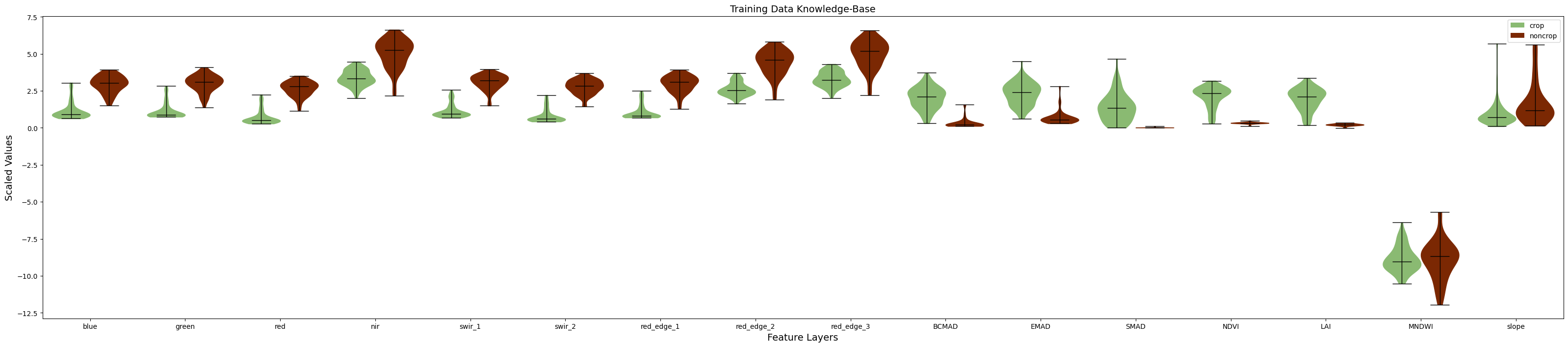
As you can see, a number of our features show good separation between the crop and non-crop classes. For example, the red, green, blue, swir, red edge 1, NDVI, and MNDWI features all have very different distributions between the classes. This is a good indication that our model will possess the right features for distinguishing between crop and non-crop later on in the workflow.

Feature Importance

Here we extract classifier estimates of the relative importance of each feature for training the classifier. This is useful for potentially selecting a subset of input bands/variables for model training/classification (i.e. optimising feature space). However, in this case, we are not selecting a subset of features, but rather just trying to understand the importance of each feature. This can help us not only understand our classes better (e.g. what kinds of measurements are indicative of cropland areas), but can also lead to further improvements to the model.

Sklearn has good documentation on different methods for feature selection.

Results will be presented in ascending order with the most important features listed last. Importance is reported as a relative fraction between 0 and 1. These importances are based on how much a given feature, on average, decreases the weighted Gini impurity.

model=RandomForestClassifier(random_state=42)
model.fit(X, y.values.ravel());

order = np.argsort(model.feature_importances_)

plt.figure(figsize=(15,5))
plt.bar(x=np.array(column_names[1:])[order],
        height=model.feature_importances_[order])
plt.gca().set_ylabel('Importance', labelpad=10)
plt.gca().set_xlabel('Feature', labelpad=10)
plt.tight_layout()

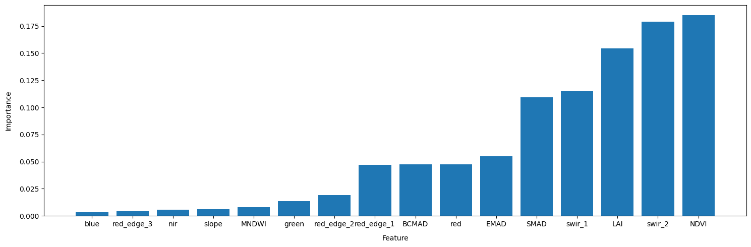
According to the the feature importance method of the RandomForestClassifier we fitted to our data, the LAI, NDVI and swir_2 band are our most important features for discriminating between crop and non-crop samples in Egypt.

Principal Component Analysis

The code below will calculate and plot the first two principal components of our training dataset. This will transform our dataset with lots of variables (16 features) into a dataset with fewer variables, this allows us to visualise our dataset in a relatively intuitive and straightforward manner.

The first step is to standardise our data to express each feature layer in terms of mean and standard deviation. This is necessary because principal component analysis is quite sensitive to the variances of the initial variables. If there are large differences between the ranges of initial variables, those variables with larger ranges will dominate over those with small ranges (For example, a variable that ranges between 0 and 100 will dominate over a variable that ranges between 0 and 1), which will lead to biased results. So, transforming the data to comparable scales can prevent this problem. We do this using sklearn’s StandardScalar function which will normalise the values in an array to the array’s mean and standard deviation via the formula:

\begin{align*} z = \frac{x-u}{s} \end{align*}

where \(u\) is the mean and \(s\) is the standard deviation.

# Compute the mean and variance for each feature
X_scaled = scaler.transform(X)

Conduct the PCAs

#two components
pca2 = PCA(n_components=2)
pca2_fit = pca2.fit_transform(X_scaled)
#three PCA components
pca3 = PCA(n_components=3)
pca3_fit = pca3.fit_transform(X_scaled)

#add back to df
pca2_df = pd.DataFrame(data = pca2_fit,
                      columns = ['PC1', 'PC2'])
pca3_df = pd.DataFrame(data = pca3_fit,
                      columns = ['PC1', 'PC2', 'PC3'])

# concat with classes
result2 = pd.concat([pca2_df, pd.DataFrame({'class':model_input[:,0]})], axis=1)
result3 = pd.concat([pca3_df, pd.DataFrame({'class':model_input[:,0]})], axis=1)

Now we can print the amount of variance explained by the two- and three-component PCAs.

a2,b2 = pca2.explained_variance_ratio_
a3,b3,c3 = pca3.explained_variance_ratio_
print("Variance explained by two principal components = " + str(round((a2+b2)*100, 2))+" %")
print("Variance explained by three principal components = " + str(round((a3+b3+c3)*100, 2))+" %")

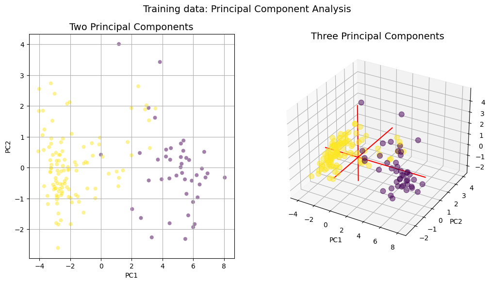
Variance explained by two principal components = 83.43 %
Variance explained by three principal components = 89.91 %

Plot both 2 & 3 principal components

if len(result2) > 5000:
    result2=result2.sample(n=5000)
if len(result3) > 5000:
    result3=result3.sample(n=5000)

fig = plt.figure(figsize=(12,6))
fig.suptitle('Training data: Principal Component Analysis', fontsize=14)

# First subplot
ax = fig.add_subplot(1, 2, 1)
scatter1=sns.scatterplot(x="PC1", y="PC2",
           data=result2,
           hue='class',
           hue_norm=tuple(np.unique(result2['class'])),
           palette='viridis',
           legend=False,
           alpha=0.5,
           ax=ax
          )

ax.set_title('Two Principal Components', fontsize=14)
ax.grid(True)

# Second subplot
ax = fig.add_subplot(1, 2, 2, projection='3d')
scatter2 = ax.scatter(result3['PC1'], result3['PC2'], result3['PC3'],
                      c=result3['class'], s=60, alpha=0.5)

# make simple, bare axis lines through space:
xAxisLine = ((min(result3['PC1']), max(result3['PC1'])), (0, 0), (0,0))
ax.plot(xAxisLine[0], xAxisLine[1], xAxisLine[2], 'r')
yAxisLine = ((0, 0), (min(result3['PC2']), max(result3['PC2'])), (0,0))
ax.plot(yAxisLine[0], yAxisLine[1], yAxisLine[2], 'r')
zAxisLine = ((0, 0), (0,0), (min(result3['PC3']), max(result3['PC3'])))
ax.plot(zAxisLine[0], zAxisLine[1], zAxisLine[2], 'r')

ax.set_title('Three Principal Components', fontsize=14)
ax.set_xlabel("PC1")
ax.set_ylabel("PC2")
ax.set_zlabel("PC3");

Conclusions

The purpose of this notebook was to inspect our training data to determine its appropriateness for classifying cropland areas. The excellent separation between our two datasets shown in the violin and PCA plots above suggests we have enough training data and the right feature layers to proceed with our classification problem.

Recommended next steps

To continue working through the notebooks in this Scalable Machine Learning on the ODC workflow, go to the next notebook 3_Train_fit_evaluate_classifier.ipynb.

1. Extracting_training_data

2. Inspect_training_data (this notebook)

3. Evaluate_optimize_fit_classifier

4. Classify_satellite_data

5. Object-based_filtering

---

Additional information

License: The code in this notebook is licensed under the Apache License, Version 2.0. Digital Earth Africa data is licensed under the Creative Commons by Attribution 4.0 license.

Contact: If you need assistance, please post a question on the Open Data Cube Slack channel or on the GIS Stack Exchange using the open-data-cube tag (you can view previously asked questions here). If you would like to report an issue with this notebook, you can file one on Github.

Last Tested:

from datetime import datetime
datetime.today().strftime('%Y-%m-%d')

'2023-08-14'