Object-based filtering of pixel classifications

Keywords data methods; image segmentation, data methods; GEOBIA

Background

Geographic Object-Based Image Analysis (GEOBIA), aims to group pixels together into meaningful image-objects. There are two advantages to a GEOBIA workflow: one, we can reduce the ‘salt and pepper’ effect typical of classifying pixels; and two, we can increase the computational efficiency of our workflow by grouping pixels into fewer, larger, but more meaningful objects. A review of the emerging trends in GEOBIA can be found in Chen et al. (2017).

Description

In this notebook, we take the pixel-based classifications generated in the 4_Classify_satellite_data.ipynb notebook, and filter the classifications by image-objects. To do this, we first need to conduct image segmentation using the function skimage.segmentation.quickshift. The image segmentation is conducted on the NDVI layer output in the previous notebook. To filter the pixel observations, we assign to each segment the majority (mode) pixel classification using the scipy.ndimage.measurements import _stats module.

1. Run the image segmentation

2. Visualize the segments

3. Calculate the mode statistic for each segment

4. Write the new object-based classification to disk as a COG

5. Plot the result

---

Getting started

To run this analysis, run all the cells in the notebook, starting with the “Load packages” cell.

Load Packages

import scipy
import xarray as xr
import rioxarray
import numpy as np
import matplotlib.pyplot as plt
from datacube.utils.cog import write_cog
from scipy.ndimage._measurements import _stats
from skimage.segmentation import quickshift

Analysis Parameters

• pred_tif: The path and name of the prediction GeoTIFF output in the previous notebook.

• tif_to_seg: The geotiff to use as an input to the image segmentation, in the default example this was an NDVI layer output in the last notebook.

• results: A folder location to store the classified GeoTIFFs.

pred_tif = 'results/prediction.tif'

tif_to_seg = 'results/NDVI.tif'

results = 'results/'

Generate an object-based classification

Run image segmentation

# Convert our mean NDVI xarray into a numpy array
ndvi = rioxarray.open_rasterio(tif_to_seg).squeeze().values

# Calculate the segments
segments = quickshift(ndvi,
                      kernel_size=2,
                      convert2lab=False,
                      max_dist=4,
                      ratio=1.0)

Visualise segments

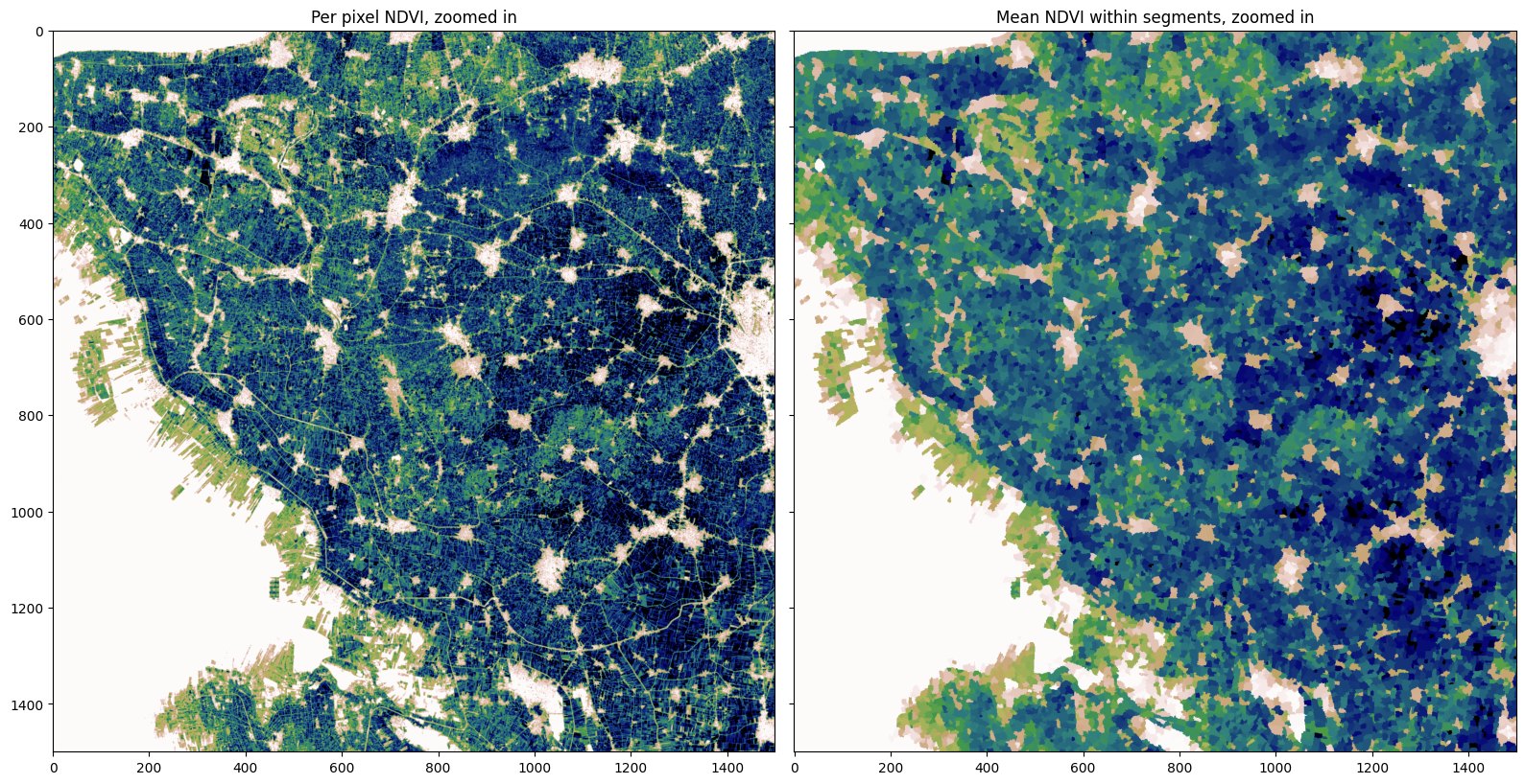
To help us visualize the segments, we can calculate the zonal mean NDVI for each segment and then we’ll plot a zoomed in section of the region

segments_zonal_mean_qs = scipy.ndimage.mean(input=ndvi,
                                            labels=segments,
                                            index=segments)

fig,ax=plt.subplots(1,2, figsize=(16,8), sharey=True)
ax[0].imshow(ndvi[1000:2500,1000:2500], cmap='gist_earth_r', vmin=0.1, vmax=0.7)
ax[1].imshow(segments_zonal_mean_qs[1000:2500,1000:2500], cmap='gist_earth_r', vmin=0.1, vmax=0.7)
ax[0].set_title('Per pixel NDVI, zoomed in');
ax[1].set_title('Mean NDVI within segments, zoomed in')
plt.tight_layout();

Open pixel-based predictions

pred = rioxarray.open_rasterio(pred_tif).squeeze().drop_vars('band')

Calculate mode

Within each segment, the majority classification is calculated and assigned to that segment.

count, _sum =_stats(pred, labels=segments, index=segments)
mode = _sum > (count/2)
mode = xr.DataArray(mode,  coords=pred.coords, dims=pred.dims, attrs=pred.attrs).astype(np.int16)

Write result to disk

write_cog(mode, results+ 'prediction_object.tif', overwrite=True)

PosixPath('results/prediction_object.tif')

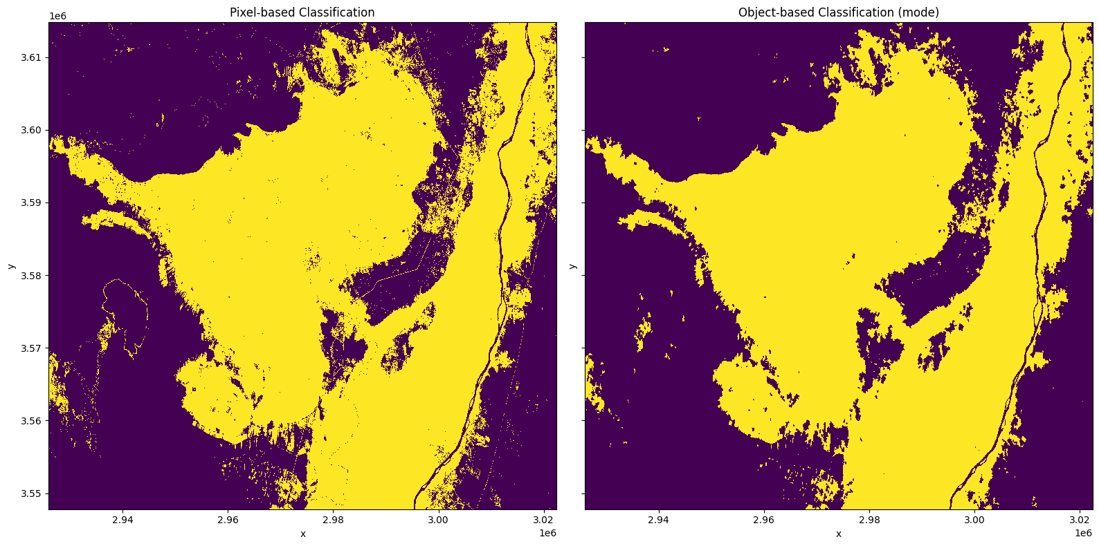
Plot result

Below we plot the the pixel-based classification alongside the newly created object-based classification. You can see the ‘salt and pepper’ effect of individual pixels being classified as crop has been removed in the object based classification, resulting in a ‘cleaner’ classification.

fig, axes = plt.subplots(1, 2, sharey=True, figsize=(16, 8))
pred.plot(ax=axes[0], add_colorbar=False)
mode.plot(ax=axes[1], add_colorbar=False)
axes[0].set_title('Pixel-based Classification')
axes[1].set_title('Object-based Classification (mode)')
plt.tight_layout();

Recommended next steps

This is the last notebook in the Scalable Machine Learning on the ODC workflow! To revist any of the other notebooks, use the links below.

1. Extracting_training_data

2. Inspect_training_data

3. Evaluate_optimize_fit_classifier

4. Classify_satellite_data

5. Object-based_filtering (this notebook)

---

Additional information

License: The code in this notebook is licensed under the Apache License, Version 2.0. Digital Earth Africa data is licensed under the Creative Commons by Attribution 4.0 license.

Contact: If you need assistance, please post a question on the Open Data Cube Slack channel or on the GIS Stack Exchange using the open-data-cube tag (you can view previously asked questions here). If you would like to report an issue with this notebook, you can file one on Github.

Last Tested:

from datetime import datetime
datetime.today().strftime('%Y-%m-%d')

'2023-08-11'