odc-stac
Why use odc-stac?
odc-stac allows you to load datasets from Digital Earth Africa in your own computing environment. While Digital Earth Africa provides users with a managed Jupyter Lab environment with limited computing resources, i.e. the Analysis Sandbox, for interacting with and analyzing Digital Earth Africa’s earth observation data, this computing environment has these drawbacks:
Being a managed environment, the user is limited in how much they can customize the Analysis Sandbox to suit their needs. If you wish to use modules/packages outside the pre-loaded packages in the default Analysis Sandbox, you will need to reinstall them everytime you start up your Analysis Sandbox environment as they do not persist.
Carrying out an analysis over a large area like an entire country can be challenging even with the larger 32GB environment provided.
Accessing datasets from sources other than Digital Earth Africa requires downloading the data onto your local machine, then uploading the data into the Analysis Sandbox.
The odc-stac is a suitable alternative to using the Analyis Sandbox, because it is a set of tools that converts STAC metadata to the Open Data Cube data model. odc-stac allows you to load STAC items into xarray.Datasets, and process them locally or disribute data loading and computation with Dask.
Table 1: Comparison between ODC and STAC concepts.
STAC |
ODC |
Description |
|---|---|---|
Collection of observations across space and time |
||
Single observation (specific time and place), multi-channel |
||
Component of a single observation |
||
Pixel plane within a multi-plane asset |
||
Alias |
Refer to the same band by different |
Digital Earth Africa stores a range of data products on Amazon Web Service’s Simple Cloud Storage (S3) with free public access. Digital Earth Africa also provides a SpatioTemporal Asset Catalog (STAC) endpoint for listing or searching the metadata, e.g. bounding box (area of interest coordinates), collection and date and time, for this archive here: https://explorer.digitalearth.africa/stac. Using the STAC endpoint provided, the odc-stac module gives you the ability to access Digital Earth
Africa’s earth observation data outside of the Analysis Sandbox, on your own resources, whether locally or on a cloud service such as Amazon Web Services (AWS), from the python environment of your choice, in the same format (as an xarray.Dataset) as you would in the Analysis Sandbox. You can also use odc-stac to load other STAC compliant earth observation data as an xarray.Dataset.
Getting started with odc-stac
Instructions on how to install the odc-stac module into your Python environment are provided here.
Example notebooks on how you can use odc-stac can be viewed here:
To download and run these notebooks, visit the odc-stac Github repository.
For more on the odc-stac see the odc-stac documentation and the odc-stac Github repository.
Complete example for Digital Earth Africa
This example demonstrates a simple analysis workflow based on the Digital Earth Africa Annual Landsat-8 and Landsat-9 GeoMAD product. In this example, we will load the Annual Landsat-8 and Landsat-9 GeoMAD data using the odc.stac stac_load function then calculate the Modified Normalized Difference Water Index (MNDWI). We will then plot the results of the water classification of the MNDWI index.
Note: To run this example outside the Digital Earth Africa Analysis Sandbox, download this example as a Jupyter notebook and the get_product_config.py Python script.
Load Packages
[1]:
import pprint

import matplotlib.pyplot as plt
import numpy as np
import seaborn as sns
from get_product_config import get_product_config
from pystac_client import Client

from odc.stac import configure_rio, stac_load
Set Collection Configuration
The purpose of the configuration dictionary is to supply some optional STAC extensions that a data source might be missing. This missing information includes, pixel data type, nodata value, unit attribute and band aliases. The configuration dictionary is passed to the odc.stac.load stac_cfg= parameter in order to supply the missing information at load time.
The configuration is per collection per asset and is determined from the product’s definition. The Annual Landsat-8 and Landsat-9 GeoMAD product definition is available at https://explorer.digitalearth.africa/products/gm_ls8_ls9_annual.
[2]:
product_name = "gm_ls8_ls9_annual"
# Set the profile to specify that the product is a Digital Earth Africa product.
profile = "deafrica"
config = get_product_config(product_name, profile)
pprint.pprint(config)
{'gm_ls8_ls9_annual': {'aliases': {'BCDEV': 'BCMAD',
                                   'EDEV': 'EMAD',
                                   'SDEV': 'SMAD',
                                   'band_2': 'SR_B2',
                                   'band_3': 'SR_B3',
                                   'band_4': 'SR_B4',
                                   'band_5': 'SR_B5',
                                   'band_6': 'SR_B6',
                                   'band_7': 'SR_B7',
                                   'bcdev': 'BCMAD',
                                   'bcmad': 'BCMAD',
                                   'blue': 'SR_B2',
                                   'count': 'COUNT',
                                   'edev': 'EMAD',
                                   'emad': 'EMAD',
                                   'green': 'SR_B3',
                                   'nir': 'SR_B5',
                                   'red': 'SR_B4',
                                   'sdev': 'SMAD',
                                   'smad': 'SMAD',
                                   'swir_1': 'SR_B6',
                                   'swir_2': 'SR_B7'},
                       'assets': {'BCMAD': {'data_type': 'float32',
                                            'nodata': 'NaN',
                                            'unit': '1'},
                                  'COUNT': {'data_type': 'uint16',
                                            'nodata': 0,
                                            'unit': '1'},
                                  'EMAD': {'data_type': 'float32',
                                           'nodata': 'NaN',
                                           'unit': '1'},
                                  'SMAD': {'data_type': 'float32',
                                           'nodata': 'NaN',
                                           'unit': '1'},
                                  'SR_B2': {'data_type': 'uint16',
                                            'nodata': 0,
                                            'unit': '1'},
                                  'SR_B3': {'data_type': 'uint16',
                                            'nodata': 0,
                                            'unit': '1'},
                                  'SR_B4': {'data_type': 'uint16',
                                            'nodata': 0,
                                            'unit': '1'},
                                  'SR_B5': {'data_type': 'uint16',
                                            'nodata': 0,
                                            'unit': '1'},
                                  'SR_B6': {'data_type': 'uint16',
                                            'nodata': 0,
                                            'unit': '1'},
                                  'SR_B7': {'data_type': 'uint16',
                                            'nodata': 0,
                                            'unit': '1'}}}}
Set AWS Configuration
Digital Earth Africa data is stored on S3 in Cape Town, Africa. To load the data, we must configure rasterio with the appropriate AWS S3 endpoint. This can be done with the odc.stac.configure_rio function. Documentation for this function is available at https://odc-stac.readthedocs.io/en/latest/_api/odc.stac.configure_rio.html#odc.stac.configure_rio.
The configuration below must be used when loading any Digital Earth Africa data through the STAC API.
[3]:
configure_rio(
    cloud_defaults=True,
    aws={"aws_unsigned": True},
    AWS_S3_ENDPOINT="s3.af-south-1.amazonaws.com",
)
Connect to the Digital Earth Africa STAC Catalog
[4]:
# Open the stac catalogue.
catalog = Client.open("https://explorer.digitalearth.africa/stac")
Find STAC Items to Load
Define query parameters
Note: The Annual Landsat-8 and Landsat-9 GeoMAD composite is available for the years 2021 - present.
One way to set the study area/bounding box is to set a central latitude and longitude coordinate pair, (central_lat, central_lon), then specify how many degrees to include either side of the central latitude and longitude, known as the buffer. Together, these parameters specify a square study area, as shown below:

[5]:
# Set the central latitude and longitude.
central_lat = -5.9460
central_lon = 35.5188

# Set the buffer to load around the central coordinates.
buffer = 0.03

# Compute the bounding box for the study area
study_area_lat = (central_lat - buffer, central_lat + buffer)
study_area_lon = (central_lon - buffer, central_lon + buffer)

# Set the bounding box.
# [xmin, ymin, xmax, ymax] in latitude and longitude (EPSG:4326).
bbox = [study_area_lon[0], study_area_lat[0], study_area_lon[1], study_area_lat[1]]
[6]:
# Set a start and end date.
start_date = "2021"
end_date = "2021"

# Set the STAC collections.
collections = [product_name]
Construct a query and get items from the Digital Earth Africa STAC Catalog
[7]:
# Build a query with the set parameters
query = catalog.search(
    bbox=bbox, collections=collections, datetime=f"{start_date}/{end_date}"
)

# Search the STAC catalog for all items matching the query
items = list(query.get_items())
print(f"Found: {len(items):d} datasets")
Found: 1 datasets
Load the GeoMAD data
In this step, we specify the desired coordinate system, resolution (here 30m), and bands to load. We will load 2 spectral satellite bands: green and swir_1. Since the band aliases are contained in the config dictionary, bands can be loaded using these aliases instead of the band number e.g. "swir_1" instead of "SR_B6".
We also pass the bounding box to the stac_load function to only load the requested data. The data will be lazy-loaded with dask, meaning that is won’t be loaded into memory until necessary, such as when it is displayed.
[8]:
# Specify the bands to load, the desired crs and resolution.
measurements = ("green", "swir_1")
crs = "EPSG:6933"
resolution = 30
[9]:
# Load the dataset.
ds_ls = stac_load(
    items,
    bands=measurements,
    crs=crs,
    resolution=resolution,
    chunks={},
    stac_cfg=config,
    bbox=bbox,
).squeeze()
[10]:
# View the xarray.Dataset.
ds_ls
[10]:
<xarray.Dataset>
Dimensions:      (y: 255, x: 194)
Coordinates:
  * y            (y) float64 -7.534e+05 -7.534e+05 ... -7.61e+05 -7.61e+05
  * x            (x) float64 3.424e+06 3.424e+06 3.424e+06 ... 3.43e+06 3.43e+06
    spatial_ref  int32 6933
    time         datetime64[ns] 2021-01-01
Data variables:
    green        (y, x) uint16 dask.array<chunksize=(255, 194), meta=np.ndarray>
swir_1 (y, x) uint16 dask.array<chunksize=(255, 194), meta=np.ndarray>Compute the MNDWI index
After loading the data, you can perform standard xarray operations, such as calculating the Modified Normalized Difference Water Index (MNDWI).
Note: The
.compute()method triggers Dask to load the data into memory.
[11]:
# Normalize the data by dividing the data by 10,000.
ds_ls = ds_ls / 10000
# Calculate the MNDWI index.
ds_ls["MNDWI"] = (ds_ls.green - ds_ls.swir_1) / (ds_ls.green + ds_ls.swir_1)
# Convert the xarray.Dataset to a DataArray.
mndwi = ds_ls.MNDWI.compute()
CPLReleaseMutex: Error = 1 (Operation not permitted)
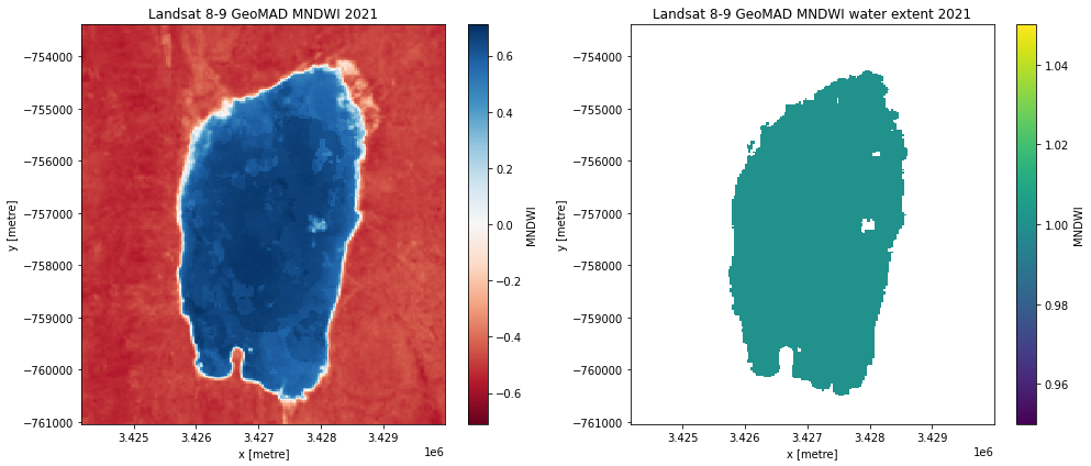
If a pixel’s MNDWI value is greater than 0, i.e. MNDWI>0 then the pixel is classified as water.
[12]:
water_mndwi = mndwi.where(mndwi > 0.5, np.nan)
water_mndwi = water_mndwi.where(np.isnan(water_mndwi), 1)
Plot the MNDWI and MNDWI water extents
[13]:
# Plot.
fig, ax = plt.subplots(1, 2, figsize=(14, 6))
mndwi.plot(ax=ax[0], cmap="RdBu")
water_mndwi.plot(ax=ax[1])

ax[0].set_title("Landsat 8-9 GeoMAD MNDWI 2021")
ax[1].set_title("Landsat 8-9 GeoMAD MNDWI water extent 2021")
plt.tight_layout();