Wetlands Insight Tool
Keywords: data used; landsat 5, data used; landsat 7, data used; landsat 8, data used; WOfS, data used; fc_ls, interactive, analysis; Wetlands insight tool, wetlands
Background
According to Wetlands International, Africa’s wetlands ecosystems are estimated to cover 131 million hectares, and include some of the most productive and biodiverse ecosystems in the world. They provide a host of ecosystem services that contribute to human well-being through nutrition, water supply and purification, climate and flood regulation, coastal protection, feeding and nesting sites for animals, recreational opportunities
and increasingly, tourism. As such, the health of wetland ecosystems has been identified as an important metric for the Sustainable Development Goals (6.6.1 Change in the extent of water-related ecosystems over time).
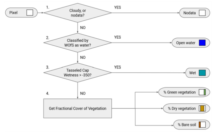
The Wetlands Insight Tool (WIT) provides insights into a wetland’s seasonal and interannual dynamics. WIT is a spatiotemporal summary of a wetland that combines multiple datasets derived from the Landsat archive held within DE Africa. Fractional cover, WOfS, and Landsat surface reflectance data are retrieved from DE Africa’s ODC and combined to produce a stack plot describing the percentage of a wetland polygon as vegetation fractional cover, open water, and wet vegetation
through time. The figure below (on the right) summaries the classification logic of the Wetlands Insight Tool.
The animation below shows an example of WIT over Lake Korienze in Mali. The WIT plot shows the percentage of the region that is covered (in order) in open water, wet soil, green vegetation, dry vegetation, and bare soil
Example of WIT over Lake Korienze, Mali |
Classification logic of the Wetlands Insight Tool |
|---|---|
|
|
Reference
Dunn et al. (2019) Developing a Tool for Wetland Characterization Using Fractional Cover, Tasseled Cap Wetness And Water Observations From Space
Description
This interactive notebook will run the Wetlands Insight Tool for the area encompassed by a polygon drawn on the interactive map.
Set the parameters for the Wetlands Insight Tool
Draw a polygon using the interactive jupyter widget
Run the WIT tool, resulting in a stacked plot of fractional cover, wetness, and water
Instructions for running the application
Make sure you read the Analysis Parameters section below so you undertand the different parameters of the Wetlands Insight Tool, then run the cell containing the wit_app() function to get started.
Use the drop-down boxes to set the parameters, draw a polygon on the interactive map over the region of interest, and then hit the Run button to begin the anlaysis. Print statements will appear on the right hand side of the app signifying the progress of the anlaysis. For more detailed progress indicators use the Dask Dashboard hyperlink that appears after you hit the run button. Note, depending on the size of the polygon drawn, and the length of time of the analysis, WIT can take a long
time to run. Once the analysis has finished, a stackplot will be plotted at the bottom of the application.
If you wish to alter the parameters and re-run the analysis over the same polygon, simply change the parameters and hit the run button again (make sure the previous run has finished before you hit the run button a second time).
If anything goes wrong with the interactvive widget and/or errors start printing on the right-hand side of the app, then restart the notebook kernel: Kernel –> Restart Kernel and Clear All Outputs
Analysis Parameters
Map Overlay: A number of overlay map layers, which can help guide polygon drawing. Options include ESRI World Imagery, the 2020 Sentinel-2 Geomedian, or the 2020 WOfS annual frequency summary. This parameter defaults to ‘None’.Start Date: The starting date of the analysis, in format DD-MM-YYYYEnd Date: The ending date of the analysis, in format DD-MM-YYYYMinimum Good Data: A number between 0 and 1 (e.g.0.85) indicating the minimum percentage of good quality pixels required for a satellite observation to be loaded and therefore included in the WIT plot. This number should, at a minimum, be set to 0.85 to limit biases in the result if not resampling the time-series. If resampling the data using the parameterResample Frequency, then setting this number to 0 (or a low float number) is acceptable.Resampling Frequency: Option for resampling time-series of input datasets. This option is useful for either smoothing the WIT plot, or because the area of analysis is larger than a scene width and therefore requires composites. Options include any string accepted byxarray.resample(time=); e.g.1M= 1 month,3M= 3 months,Q-DEC= quarterly starting in December. To turn off resampling set this parameter toNone. The resampling method used is .max(), hence the resulting plots will show the maximum extent of each variable during the resampled interval.Output CSV: To output a .csv file with the values of the WIT plot, enter a file name e.g.output_WIT.csvOutput Plot: To output a .png copy of the WIT stackplot, enter a file name e.g.output_WIT.png
[1]:
from deafrica_tools.app.wetlandsinsighttool import wit_app

wit_app()
[1]:
Additional information
License The code in this notebook is licensed under the Apache License, Version 2.0.
Digital Earth Africa data is licensed under the Creative Commons by Attribution 4.0 license.
Contact If you need assistance, please post a question on the DE Africa Slack channel or on the GIS Stack Exchange using the open-data-cube tag (you can view previously asked questions here).
If you would like to report an issue with this notebook, you can file one on Github.
Compatible datacube version
[2]:
import datacube
print(datacube.__version__)
1.8.19
Last Tested:
[3]:
from datetime import datetime
datetime.today().strftime('%Y-%m-%d')
[3]:
'2024-11-05'