Identifying active irrigated cropping
Products used: ls8_st, ls8_sr, crop_mask, ERA5 Climate Data
Keywords data used; landsat 8, datasets; landsat 8, surface temperature, data used; ERA5, datasets; ERA5, climate, temperature
Background
One of the well-known measures of plant health is canopy temperature. In conditions with limited water, it can be assumed transpiration decreases and plant temperature subsequently increases. This can often happen during periods of moisture stress in dryland (rainfed) cropping systems but can be overcome by water application in irrigated cropping systems.
In the field, canopy temperatures can be measured by handheld radiometers. This sort of data is used at a small scale to examine crop health and yield under a variety of conditions. At larger scales, an alternative method is to use surface temperature detected by satellites such as Landsat 8 to calculate similar metrics. In this notebook, we will use \(\Delta T\) to differentiate between dryland and irrigated cropland, where \(\Delta T\) is:
\begin{equation} \Delta T = T_c - T_a \end{equation}
where
\(T_c\) is crop canopy temperature
\(T_a\) is air temperature
Lower \(\Delta T\) is associated with higher rates of transpiration as evaporative cooling from transpiration cools the canopy, while higher \(\Delta T\) indicates lower rates of transpiration and thereby moisture stress.
In this case, we will use measurements of air temperature modelled by ERA5 to approximate \(T_a\) and the Landsat surface temperature product to approximate \(T_c\).
Description
In this notebook, we calculate \(\Delta T\) and visualise over irrigated areas.
The following steps are taken:
Load Landsat 8 Surface Temperature data
Load ERA5 “Air temperature at 2 metres” data for the same area of interest
Calculate \(\Delta T\)
Visualise \(\Delta T\)
Use a simple cluster analysis to differentiate between irrigated and dryland cropping.
Map irrigated cropping within the area of interest.
Load packages
[1]:
%matplotlib inline
import warnings
warnings.filterwarnings("ignore", category=FutureWarning)

import datacube
import numpy as np
import xarray as xr
import geopandas as gpd
import matplotlib.pyplot as plt
from odc.geo.xr import xr_reproject
from matplotlib.colors import ListedColormap

from deafrica_tools.load_era5 import load_era5
from deafrica_tools.datahandling import load_ard, mostcommon_crs
from deafrica_tools.plotting import rgb, display_map
from odc.geo.geom import Geometry
from deafrica_tools.bandindices import calculate_indices
from deafrica_tools.classification import sklearn_flatten, sklearn_unflatten
from sklearn.cluster import KMeans
from sklearn.preprocessing import StandardScaler
from deafrica_tools.areaofinterest import define_area
Connect to the datacube
[2]:
dc = datacube.Datacube(app="Landsat_ST")
Analysis parameters
This analysis focuses on cropland in Sudan. The western portion of the area of interest appear irrigated, as it is serviced by canals on close inspection, and vegetation is greener than surrounding landscape features. The eastern portion of the area is mostly dryland cropping.
Select location
To define the area of interest, there are two methods available:
By specifying the latitude, longitude, and buffer. This method requires you to input the central latitude, central longitude, and the buffer value in square degrees around the center point you want to analyze. For example,
lat = 10.338,lon = -1.055, andbuffer = 0.1will select an area with a radius of 0.1 square degrees around the point with coordinates (10.338, -1.055).Alternatively, you can provide separate buffer values for latitude and longitude for a rectangular area. For example,
lat = 10.338,lon = -1.055, andlat_buffer = 0.1andlon_buffer = 0.08will select a rectangular area extending 0.1 degrees north and south, and 0.08 degrees east and west from the point(10.338, -1.055).For reasonable loading times, set the buffer as
0.1or lower.By uploading a polygon as a
GeoJSON or Esri Shapefile. If you choose this option, you will need to upload the geojson or ESRI shapefile into the Sandbox using Upload Files button in the top left corner of the Jupyter Notebook interface. ESRI shapefiles must be uploaded with all the related files
 (.cpg, .dbf, .shp, .shx). Once uploaded, you can use the shapefile or geojson to define the area of interest. Remember to update the code to call the file you have uploaded.
To use one of these methods, you can uncomment the relevant line of code and comment out the other one. To comment out a line, add the "#" symbol before the code you want to comment out. By default, the first option which defines the location using latitude, longitude, and buffer is being used.
[3]:
# Method 1: Specify the latitude, longitude, and buffer
aoi = define_area(lat=13.8489, lon=33.822, buffer=0.125)

# Method 2: Use a polygon as a GeoJSON or Esri Shapefile.
# aoi = define_area(vector_path='aoi.shp')

#Create a geopolygon and geodataframe of the area of interest
geopolygon = Geometry(aoi["features"][0]["geometry"], crs="epsg:4326")
geopolygon_gdf = gpd.GeoDataFrame(geometry=[geopolygon], crs=geopolygon.crs)

# Get the latitude and longitude range of the geopolygon
lat_range = (geopolygon_gdf.total_bounds[1], geopolygon_gdf.total_bounds[3])
lon_range = (geopolygon_gdf.total_bounds[0], geopolygon_gdf.total_bounds[2])

# Set the range of dates for the analysis
time = ("2018-01-01", "2019-12-31")

time = ("2019-06", "2019-11")

measurements = ["surface_temperature"]
View selected location
[4]:
display_map(lon_range, lat_range)
[4]:
Load Landsat 8 Surface Temperature data
[5]:
ds_land = load_ard(
    dc=dc,
    products=["ls8_st"],
    x=lon_range,
    y=lat_range,
    time=time,
    measurements=measurements,
    skip_broken_datasets=True,
    output_crs="EPSG:6933",
    mask_filters=[("opening", 5), ("dilation", 5)],  # improve cloud-mask
    resolution=(-30, 30),
)

print(ds_land)
Using pixel quality parameters for USGS Collection 2
Finding datasets
    ls8_st
Applying morphological filters to pq mask [('opening', 5), ('dilation', 5)]
Applying pixel quality/cloud mask
Re-scaling Landsat C2 data
Loading 24 time steps
<xarray.Dataset> Size: 80MB
Dimensions:              (time: 24, y: 1034, x: 805)
Coordinates:
  * time                 (time) datetime64[ns] 192B 2019-06-05T08:03:16.92750...
  * y                    (y) float64 8kB 1.766e+06 1.766e+06 ... 1.735e+06
  * x                    (x) float64 6kB 3.251e+06 3.251e+06 ... 3.275e+06
    spatial_ref          int32 4B 6933
Data variables:
    surface_temperature  (time, y, x) float32 80MB nan nan nan ... 324.5 324.4
Attributes:
    crs:           EPSG:6933
    grid_mapping:  spatial_ref
Convert to celsius and resample to annual means
[6]:
# convert from Kelvin to Celsius
celcius_kelvin_offset = 273.15
ds_land["surface_temperature"] = ds_land.surface_temperature - celcius_kelvin_offset

# Annual surface land temp
ds_land = ds_land.mean("time")
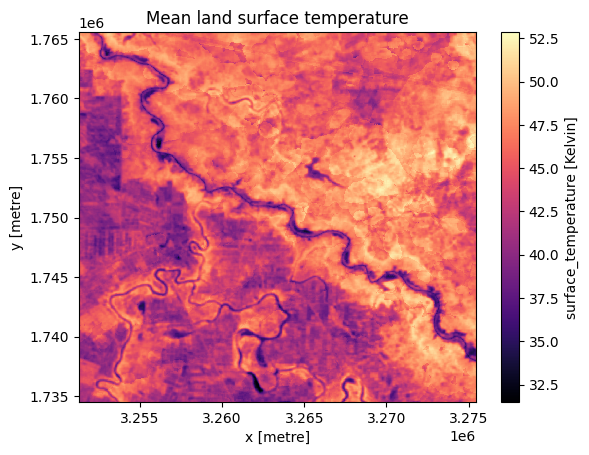
[7]:
# plot
ds_land.surface_temperature.plot.imshow(cmap="magma")
plt.title("Mean land surface temperature");
Load ERA5 Air Temperature data
While Landsat 8 will observe a given location once every few days, ERA5 provides hourly observations. As such, the next step calculates the monthly average air temperature from ERA5, using the resample and reduce_func arguments. The load_era5 function returns the temperature in Kelvin, so it must be converted to Celcius using the offset.
After calculating this, the last step is to take the average of the monthly means to get a seasonal mean air temperature, which will be used for the analysis.
[8]:
# load ERA5 air temperature at 2m height, resampled to monthly means
var = "air_temperature_at_2_metres"
ds_air = (
    load_era5(var, lat_range, lon_range, time, resample="1MS", reduce_func=np.mean)[var]
    - celcius_kelvin_offset
)
ds_air = ds_air.compute()  # bring into memory

# rename dimensions to match landsat
ds_air = ds_air.rename({"lon": "x", "lat": "y"})

# Seasonal mean air temp
ds_air = ds_air.mean("time")
Opening ERA5 Zarr dataset...
Variable: air_temperature_at_2_metres
Mapped ERA5 name: 2m_temperature
Time: 2019-06-01 to 2019-11-01
Latitude: 13.7239 to 13.9739
Longitude: 33.697 to 33.947
Selecting time range...
Normalising longitude coordinates...
Selecting AOI...
Subset size: {'time': 3696, 'latitude': 2, 'longitude': 2}
Resampling to 1MS using <function mean at 0x7f16c819b9c0>...
ERA5 loading complete.
[9]:
# plot
ds_air.plot.imshow(cmap="viridis")
plt.title("Mean air surface temperature");
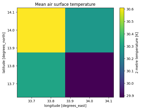
The above plots show the data has loaded correctly. Note that ERA5 has a much lower spatial resolution than Landsat 8 (approximately 31km compared to 30m) but has a much higher temporal resolution.
It is also expected that land temperature will be higher than 2 metre air temperature.
Note the land temperature estimated by Landsat 8 can seem quite high; here, it is shown in excess of 40 degrees Celsius. In this notebook, we do not have the means to validate the dataset so it is difficult to tell if the readings are accurate, or exaggerated due to inherent instrumentation error. Regardless, this is mitigated by \(\Delta T\) which looks at the difference between temperatures instead of absolute values.
Calculate \(\Delta T\)
As noted in the introduction, for this exercise we estimate \(\Delta T\) using the loaded temperature datasets in lieu of in-situ data. This can be broken down into the following steps:
Resample the air temperature to match the spatial resolution of Landsat. This is done using the
xr_reprojectfunction.Calculate the difference (\(\Delta T\)) between \(T_c\) (land temperature) and \(T_a\) (air temperature)
[10]:
ds_air = xr_reproject(src=ds_air, how=ds_land.geobox, resampling="nearest")
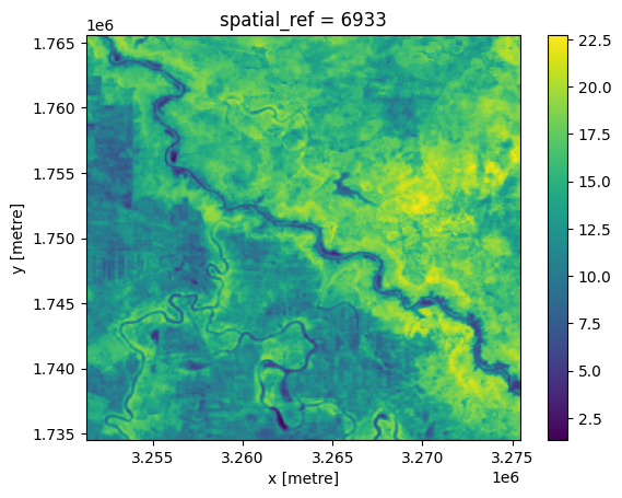
Calculate \(\Delta T\):
[11]:
deltat = ds_land.surface_temperature - ds_air
[12]:
deltat.plot.imshow();
Load Landsat-8 Surface Reflectance data and calculate NDVI
[13]:
ds_ndvi = load_ard(
    dc=dc,
    products=["ls8_sr"],
    like=ds_land.geobox,
    time=time,
    skip_broken_datasets=True,
    measurements=["red", "nir"],
)

ds_ndvi = calculate_indices(ds_ndvi, index="NDVI", satellite_mission="ls", drop=True)
Using pixel quality parameters for USGS Collection 2
Finding datasets
    ls8_sr
Applying pixel quality/cloud mask
Re-scaling Landsat C2 data
Loading 24 time steps
Dropping bands ['red', 'nir']
[14]:
ds_ndvi = ds_ndvi.median("time").squeeze()
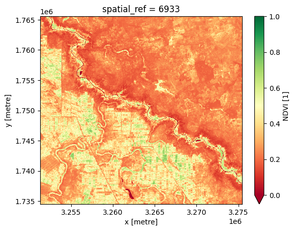
[15]:
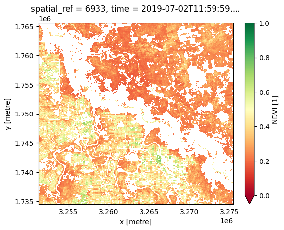
ds_ndvi.NDVI.plot.imshow(cmap="RdYlGn", vmin=0, vmax=1);
Use the Cropland extent product for masking cropping regions
We can use \(\Delta T\) to differentiate between irrigated and dryland cropping, but to do this we need to restrict our analysis to cropland and exclude other landscape features. We can do this using the cropland extent product, which we load below.
Load crop mask
[16]:
cm = dc.load(
    product="crop_mask", time="2019", measurements="filtered", like=ds_ndvi.geobox
).filtered.squeeze()
[17]:
deltat = deltat.where(cm==1)
ds_ndvi = ds_ndvi.where(cm==1)
[18]:
ds_ndvi.NDVI.plot.imshow(cmap="RdYlGn", vmin=0, vmax=1);
Identify clusters for classification
We have two variables (NDVI and \(\Delta T\)) that we’d like to use to split dryland and irrigated cropland.
We can use a cluster technique to assign the data to these classes. In this case, we’ll use k-means clustering to identify two clusters (irrigated and rainfed).
As the two variables have quite different units, we’ll need to rescale them before running the cluster analysis. This is shown in the cell below.
[19]:
# flatten the two predictors into 1-D arrays
ndvi_flat = sklearn_flatten(ds_ndvi.NDVI)
deltat_flat = sklearn_flatten(deltat)

# combine the two arrays for passing into kmeans
X = np.stack((ndvi_flat, deltat_flat), axis=0).transpose()

# rescale variables for cluster analysis
scaler = StandardScaler()
X_scaled = scaler.fit_transform(X)

# perform kmeans cluster analysis, specifying we are looking for two clusters
kmeans = KMeans(n_clusters=2, random_state=0)
kmeans.fit(X_scaled)
y_kmeans = kmeans.predict(X_scaled)

# create a lookup table for the clusters so results are reproducible
idx = np.argsort(kmeans.cluster_centers_.sum(axis=1))
lut = np.zeros_like(idx)
lut[idx] = np.arange(2)
kmeans.labels_ = lut[kmeans.labels_]
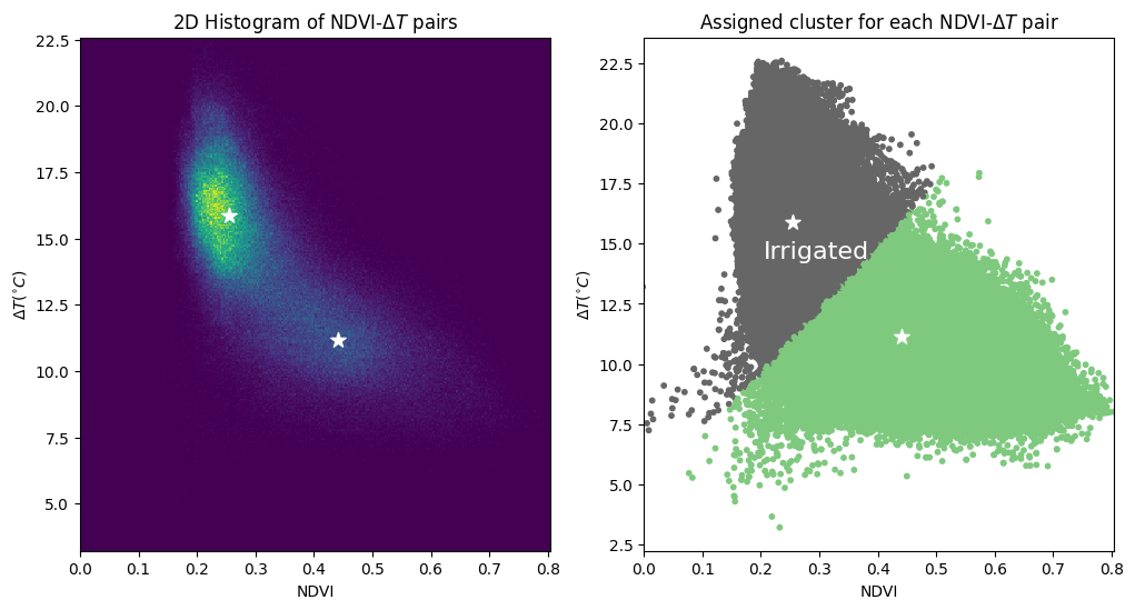
Plot the clusters
The plot below shows the 2D histogram of the NDVI-\(\Delta T\) pairs (conveying the density of points), as well as a scatter plot showing which cluster each pair was assigned to. Both plots display the centre of each cluster.
The density shows two distinct clusters that the k-means algorithm has identified in the data. We assume to cluster to the bottom-right (higher NDVI and lower \(\Delta T\)) is the irrigated cropland.
[20]:
# Get locations of kmeans cluster centres
centers_scaled = kmeans.cluster_centers_
centers = scaler.inverse_transform(centers_scaled)

# Construct the figure
fig, (ax1, ax2) = plt.subplots(1, 2, figsize=(12, 6))

ax1.hist2d(X[:, 0], X[:, 1], bins=(300, 300), cmap="viridis")
ax1.scatter(centers[:, 0], centers[:, 1], c="white", s=100, marker="*")
ax1.set_xlim(0, ds_ndvi.NDVI.max())
ax1.set_xlabel("NDVI")
ax1.set_ylabel("$\Delta T (^{\circ} C)$")
ax1.set_title("2D Histogram of NDVI-$\Delta T$ pairs")

ax2.scatter(X[:, 0], X[:, 1], c=y_kmeans, s=10, cmap="Accent")
ax2.scatter(centers[:, 0], centers[:, 1], c="white", s=100, marker="*")
ax2.set_xlim(0, ds_ndvi.NDVI.max())
ax2.set_xlabel("NDVI")
ax2.set_ylabel("$\Delta T (^{\circ} C)$")
ax2.text(
    centers[1, 0] - 0.05, centers[1, 1] - 1.5, "Irrigated", fontsize=16, color="white"
)
ax2.set_title("Assigned cluster for each NDVI-$\Delta T$ pair")

plt.show()
Apply clusters to the spatial data
[21]:
# use kmeans to predict which cluster each observation belongs to
preds_flat = kmeans.predict(X_scaled)

# unflatten predictions to return it to spatial dimensions
preds = sklearn_unflatten(preds_flat, ds_ndvi)

# irrigated (c) where cropland is true and cluster = 0
c = xr.where((cm == 1) & (preds == 1), 2, cm)
Load semi-annual geomedian to compare classification to a true-colour image.
[22]:
gm = dc.load(
    product="gm_s2_semiannual",
    like=cm.geobox,
    time=time,
    measurements=["red", "green", "blue"],
).squeeze()
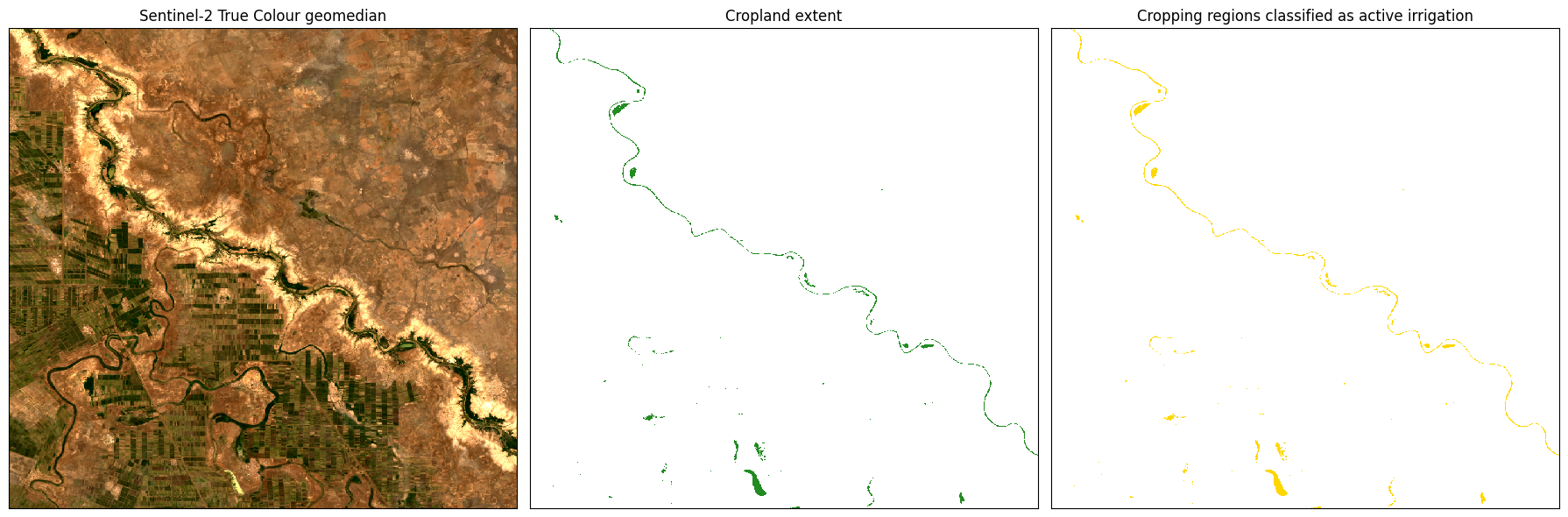
Plot result
The following produces a three-panel plot, showing the geomedian for reference, then the total cropland extent, and finally, areas classified as active irrigation in yellow.
[23]:
colours = ["white", "forestgreen", "gold"]

fig, ax = plt.subplots(1, 3, figsize=(18, 6), sharey=True)

# Geomedian
rgb(gm, index=1, ax=ax[0])
ax[0].set_title("Sentinel-2 True Colour geomedian")

# Cropland extent
cm.plot(ax=ax[1], add_colorbar=False, cmap=ListedColormap(colours[0:2]))
ax[1].set_title("Cropland extent")

# Irrigated cropping
c.plot(ax=ax[2], add_colorbar=False, cmap=ListedColormap(colours))
ax[2].set_title("Cropping regions classified as active irrigation")

# Turn axis ticks and labels off on all axes
for axis in ax:
    axis.set_xticks([])
    axis.set_yticks([])
    axis.set_xlabel("")
    axis.set_ylabel("")


plt.tight_layout();
Limitations
This method of calculating \(\Delta T\) is based on several key assumptions:
Air temperature is reasonably approximated by ERA5
Land temperature is reasonably approximated by Landsat 8 Surface Temperature
The cluster based differentiation of irrigated and dryland cropping is reliant on these two features being related these variables. This approach may be less effective in some scenarios, such as:
Wet seasons where dryland crops are experiencing low levels of moisture stress and high canopy greenness.
Cold times when \(\Delta T\) may not be a good indicator of crop moisture stress.
As always, results should be interpreted with context and care.
References
Jackson, Ray D., Kustas, William P., and Choudhury, Bhaskar J. 1988. ‘A Reexamination of the Crop Water Stress Index’. Irrig Sci 9:309-317
Additional information
License The code in this notebook is licensed under the Apache License, Version 2.0.
Digital Earth Africa data is licensed under the Creative Commons by Attribution 4.0 license.
Contact If you need assistance, please post a question on the DE Africa Slack channel or on the GIS Stack Exchange using the open-data-cube tag (you can view previously asked questions here).
If you would like to report an issue with this notebook, you can file one on Github.
Compatible datacube version
[24]:
print(datacube.__version__)
1.9.13
Last Tested:
[25]:
from datetime import datetime
datetime.today().strftime('%Y-%m-%d')
[25]:
'2026-04-30'