Detecting change in urban extent
Products used: gm_s2_annual
Keywords: data used; sentinel-2 geomedian, band index; ENDISI, urban, analysis; change detection
Background
The rate at which cities and towns grow, or the urbanisation rate, is an important indicator of the sustainability of towns and cities. Rapid, unplanned urbanisation can result in poor social, economic, and environmental outcomes due to inadequate and overburdened infrastructure and services creating congestion, worsening air pollution, and leading to a shortage of adequate housing.
The first requirement for addressing the impacts of rapid urbanisation is to accurately and regularly monitor urban expansion in order to track urban development over time. Earth Observation datasets, such as those available through the Digital Earth Africa platform provide a cost-effective and accurate means of mapping the urban extent of cities.
Description
This notebook will use Sentinel-2 annual geomedians to examine the change in urban extent between a baseline period and a more recent period. The difference in urban extent (area is square kilometres) between the two periods is calculated, along with a map highlighting the location of urban growth hotspots.
This notebook conducts the following analysis:
Load Sentinel-2 annual geomedians data over the city/region of interest
Calculate the Enhanced Normalised Difference Impervious Surfaces Index (ENDISI)
Threshold the ENDISI plots to delineate urban extent
Compare the urban extent in the baseline year to the more recent urban extent
Getting started
To run this analysis, run all the cells in the notebook, starting with the “Load packages” cell.
Load packages
Import Python packages that are used for the analysis.
[1]:
%matplotlib inline

import datacube
import numpy as np
import xarray as xr
import geopandas as gpd
import matplotlib.pyplot as plt
from matplotlib.patches import Patch
from matplotlib.colors import ListedColormap

from odc.geo.geom import Geometry
from deafrica_tools.spatial import xr_rasterize
from deafrica_tools.dask import create_local_dask_cluster
from deafrica_tools.bandindices import calculate_indices
from deafrica_tools.plotting import display_map, rgb
from deafrica_tools.datahandling import load_ard
from deafrica_tools.areaofinterest import define_area
Set up a Dask cluster
Dask can be used to better manage memory use down and conduct the analysis in parallel. For an introduction to using Dask with Digital Earth Africa, see the Dask notebook.
Note: We recommend opening the Dask processing window to view the different computations that are being executed; to do this, see the Dask dashboard in DE Africa section of the Dask notebook.
To use Dask, set up the local computing cluster using the cell below.
[2]:
create_local_dask_cluster()
Client
Client-fc1fa00b-d420-11ef-a437-1e01ca941b00
| Connection method: Cluster object | Cluster type: distributed.LocalCluster |
| Dashboard: /user/victoria@kartoza.com/proxy/8787/status |
Cluster Info
LocalCluster
c240982c
| Dashboard: /user/victoria@kartoza.com/proxy/8787/status | Workers: 1 |
| Total threads: 7 | Total memory: 59.21 GiB |
| Status: running | Using processes: True |
Scheduler Info
Scheduler
Scheduler-33268be0-c0e4-4f24-95f1-400db9e6f7e8
| Comm: tcp://127.0.0.1:40575 | Workers: 1 |
| Dashboard: /user/victoria@kartoza.com/proxy/8787/status | Total threads: 7 |
| Started: Just now | Total memory: 59.21 GiB |
Workers
Worker: 0
| Comm: tcp://127.0.0.1:45445 | Total threads: 7 |
| Dashboard: /user/victoria@kartoza.com/proxy/40025/status | Memory: 59.21 GiB |
| Nanny: tcp://127.0.0.1:33905 | |
| Local directory: /tmp/dask-scratch-space/worker-wnkeh7_2 | |
Connect to the datacube
Activate the datacube database, which provides functionality for loading and displaying stored Earth observation data.
[3]:
dc = datacube.Datacube(app='Urbanisation')
Analysis parameters
The following cell set important parameters for the analysis:
lat: The central latitude to analyse (e.g.14.283).lon: The central longitude to analyse (e.g.-16.921).buffer: The number of square degrees to load around the central latitude and longitude. For reasonable loading times, set this as0.1or lower.baseline_year: The baseline year, to use as the baseline of urbanisation (e.g.2017)analysis_year: The analysis year to analyse the change in urbanisation (e.g.2020)
Select location
To define the area of interest, there are two methods available:
By specifying the latitude, longitude, and buffer. This method requires you to input the central latitude, central longitude, and the buffer value in square degrees around the center point you want to analyze. For example,
lat = 10.338,lon = -1.055, andbuffer = 0.1will select an area with a radius of 0.1 square degrees around the point with coordinates (10.338, -1.055).Alternatively, you can provide separate buffer values for latitude and longitude for a rectangular area. For example,
lat = 10.338,lon = -1.055, andlat_buffer = 0.1andlon_buffer = 0.08will select a rectangular area extending 0.1 degrees north and south, and 0.08 degrees east and west from the point(10.338, -1.055).For reasonable loading times, set the buffer as
0.1or lower.By uploading a polygon as a
GeoJSON or Esri Shapefile. If you choose this option, you will need to upload the geojson or ESRI shapefile into the Sandbox using Upload Files button in the top left corner of the Jupyter Notebook interface. ESRI shapefiles must be uploaded with all the related files
 (.cpg, .dbf, .shp, .shx). Once uploaded, you can use the shapefile or geojson to define the area of interest. Remember to update the code to call the file you have uploaded.
To use one of these methods, you can uncomment the relevant line of code and comment out the other one. To comment out a line, add the "#" symbol before the code you want to comment out. By default, the first option which defines the location using latitude, longitude, and buffer is being used.
[4]:
# Method 1: Specify the latitude, longitude, and buffer
aoi = define_area(lat=6.854, lon=-1.392, buffer=0.035)

# Method 2: Use a polygon as a GeoJSON or Esri Shapefile.
# aoi = define_area(vector_path='aoi.shp')

#Create a geopolygon and geodataframe of the area of interest
geopolygon = Geometry(aoi["features"][0]["geometry"], crs="epsg:4326")
geopolygon_gdf = gpd.GeoDataFrame(geometry=[geopolygon], crs=geopolygon.crs)

# Get the latitude and longitude range of the geopolygon
lat_range = (geopolygon_gdf.total_bounds[1], geopolygon_gdf.total_bounds[3])
lon_range = (geopolygon_gdf.total_bounds[0], geopolygon_gdf.total_bounds[2])

# Change the years values also here
# Note: Sentinel-2 starts from 2017
baseline_year = 2017
analysis_year = 2020
View the selected location
The next cell will display the selected area on an interactive map. Feel free to zoom in and out to get a better understanding of the area you’ll be analysing. Clicking on any point of the map will reveal the latitude and longitude coordinates of that point.
[5]:
display_map(lon_range, lat_range)
[5]:
Load Sentinel-2 annual geomedians
The first step in this analysis is to load in Sentinel-2 annual geomedians for the lat_range, lon_range and time_range we provided above.
[6]:
# Create a query
query = {
    'time': (f'{baseline_year}', f'{analysis_year}'),
    'x': lon_range,
    'y': lat_range,
    'resolution': (-20, 20),
    'measurements':['swir_1','swir_2','blue','green','red'],
    'group_by': 'solar_day',

}

# Create a dataset of the requested data
geomedians = dc.load(product='gm_s2_annual',
        output_crs='EPSG:6933',
        dask_chunks={'time': 1, 'x': 750, 'y': 750},
        **query
)
Select the images from the baseline and analysis years
[7]:
#groupby year so the time dimension is converted to year
# the .mean() doesn't do anything here
geomedians=geomedians.groupby('time.year').mean()

geomedians = geomedians.sel(year=[baseline_year, analysis_year])
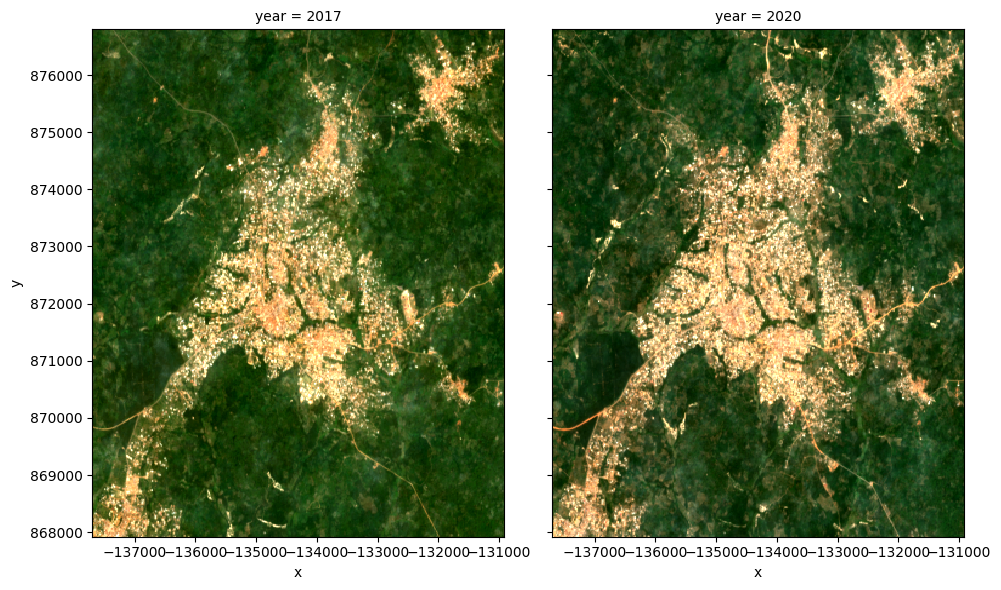
View the geomedian satellite data
We can plot the two years to visually compare them:
[8]:
rgb(geomedians, col='year')
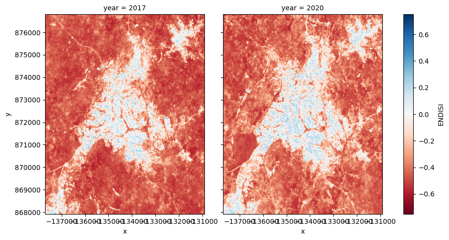
Calculate ENDISI
The Enhanced Normalized Difference Impervious Surfaces Index (ENDISI) is a recently developed urbanisation proxy that has been shown to work well in a variety of environments (Chen et al. 2020) . Like all normalised difference indicies, it has a range of [-1,1]. Note that MNDWI, swir_diff and alpha are all part of the ENDISI calculation.
ENDISI calculations are built into the calculate_indices function. We are using the Sentinel-2 geomedian, so the satellite_mission will be s2.
[9]:
# Calculate the ENDISI index
geomedians = calculate_indices(geomedians, index='ENDISI', satellite_mission='s2')
Let’s plot the ENDISI images so we can see if the urban areas are distinguishable
[10]:
geomedians.ENDISI.plot(
    col='year',
    vmin=-.75,
    vmax=0.75,
    cmap='RdBu',
    figsize=(10, 5),
    robust=True
);
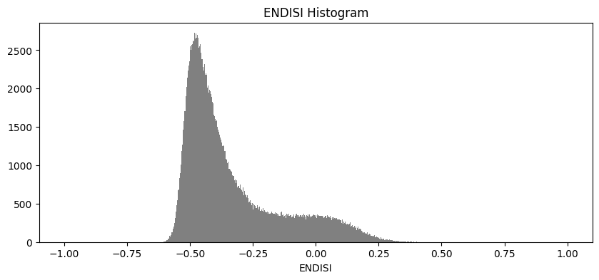
And now plot the histogram of all the pixels in the ENDISI array
[11]:
geomedians.ENDISI.plot.hist(bins=1000, range=(-1,1), facecolor='gray', figsize=(10, 4))
plt.title('ENDISI Histogram');
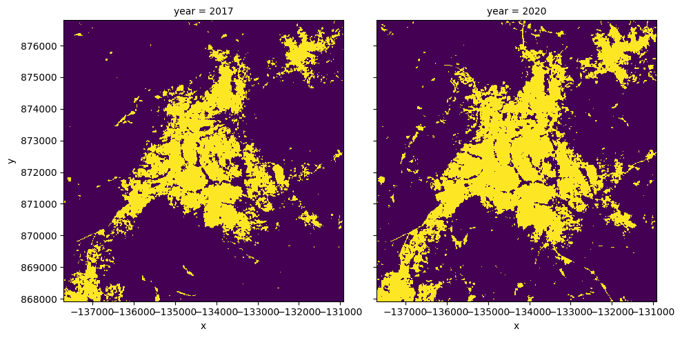
Calculate urban extent
To define the urban extent, we need to threshold the ENDISI arrays. Values above this threshold will be labelled as ‘Urban’ while values below the trhehsold will be excluded from the urban extent. We can determine this threshold a number of ways (inluding by simply manually definining it e.g. threshold=-0.1). Below, we use the Otsu method to automatically threshold the image.
Firstly, we need to fill any NaN values we have in the dataset with the mean of the dataset, otherwise the otsu threshold function will complain:
[12]:
geomedians['ENDISI'] = geomedians.ENDISI.fillna(geomedians.ENDISI.mean().values)
[13]:
from skimage.filters import threshold_otsu

threshold = threshold_otsu(geomedians.ENDISI.values)
print(round(threshold, 2))
-0.23
Apply the threshold
We apply the threshold and plot both years side-by-side.
[14]:
urban_area = (geomedians.ENDISI > threshold).astype(int)
urban_area.plot(
    col='year',
    figsize=(10, 5),
    robust=True,
    add_colorbar=False
);
Plotting the change in urban extent
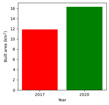
We can convert the data above into a total area for each year, then plot a bar graph.
[15]:
pixel_length = query["resolution"][1]  # in metres
area_per_pixel = pixel_length**2 / 1000**2

urban_area_km2 = urban_area.sum(dim=['x', 'y']) * area_per_pixel

# Plot the resulting area through time
fig, axes = plt.subplots(1, 1, figsize=(4, 4))
plt.bar([0, 1],
        urban_area_km2,
        tick_label=urban_area_km2.year,
        width = 0.8,
        color=['red', 'green']
       )
axes.set_xlabel("Year")
axes.set_ylabel("Built area (km$^2$)");

for y in urban_area_km2.year.values:
    print('Urban extent in '+str(y)+": "+str(round(float(urban_area_km2.sel(year=y).values),3))+' km2')
Urban extent in 2017: 11.852 km2
Urban extent in 2020: 16.285 km2
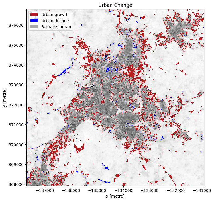
Urban growth hotspots
If we subtract the ENDISI of the baseline year from the analysis year, we can highlight regions where urban growth is occurring.
In this plot, we can see areas that have seen significant change, highlighting regions of urbanisation.
[16]:
# Calculate the change between the years
urban_change = urban_area.sel(
    year=analysis_year) - urban_area.sel(year=baseline_year)

urban_growth = urban_change.where(urban_change == 1)
urban_decline = urban_change.where(urban_change == -1)
[17]:
urban_appeared = '#b91e1e'
urban_disappeared = 'Blue'

# Plot urban extent from first year in grey as a background
plot = geomedians.ENDISI.sel(year=baseline_year).plot(size=8,
                                                      aspect=urban_area.y.size /
                                                      urban_area.y.size,
                                               cmap='Greys',
                                               add_colorbar=False)

# add urban growth and decline to the plot
urban_growth.plot(ax=plot.axes,
                  cmap=ListedColormap([urban_appeared]),
                  add_colorbar=False,
                  add_labels=False,
                  )
urban_decline.plot(ax=plot.axes,
                   cmap=ListedColormap([urban_disappeared]),
                   add_colorbar=False,
                   add_labels=False
                   )
# Add the legend
plot.axes.legend(
    [
        Patch(facecolor=urban_appeared),
        Patch(facecolor=urban_disappeared),
        Patch(facecolor='darkgrey'),
        Patch(facecolor='white')
    ],
    ['Urban growth', 'Urban decline', 'Remains urban'],
    loc='upper left'
)

plt.title('Urban Change');
Next steps
When you are done, return to the Analysis parameters section, modify some values (e.g. lat, lon or time) and rerun the analysis.
You can use the interactive map in the View the selected location section to find new central latitude and longitude values by panning and zooming, and then clicking on the area you wish to extract location values for. You can also use Google maps to search for a location you know, then return the latitude and longitude values by clicking the map.
If you’re going to change the location, you’ll need to make sure Landsat 8 data is available for the new location, which you can check at the Digital Earth Africa Explorer.
For more advanced methods of urban extent detection, see the Machine Learning with ODC notebook, which uses a decision tree to classify urban area.
Additional information
License The code in this notebook is licensed under the Apache License, Version 2.0.
Digital Earth Africa data is licensed under the Creative Commons by Attribution 4.0 license.
Contact If you need assistance, please post a question on the DE Africa Slack channel or on the GIS Stack Exchange using the open-data-cube tag (you can view previously asked questions here).
If you would like to report an issue with this notebook, you can file one on Github.
Compatible datacube version
[18]:
print(datacube.__version__)
1.8.20
Last Tested:
[19]:
from datetime import datetime
datetime.today().strftime('%Y-%m-%d')
[19]:
'2025-01-16'