GéoMAD roulant

• Produits utilisés : gm_s2_rolling, ndvi_anomaly

Mots-clés : données utilisées ; rolling geomad, données utilisées ; sentinel-2

Aperçu

L’imagerie satellite nous permet d’observer la Terre de manière répétitive et détaillée. Cependant, les données manquantes, comme les trous causés par la couverture nuageuse, peuvent rendre difficile la création d’une image complète. Afin de produire une vue unique et complète d’une certaine zone, les données satellite peuvent être consolidées, en empilant les mesures de différents moments dans le temps pour créer une image composite.

Le service Sentinel-2 Rolling GeoMAD (Geomedian et Median Absolute Deviations) de Digital Earth Africa (DE Africa) fournit des données mensuelles sur les géomédianes et les MAD calculés à l’aide d’une fenêtre mobile de 3 mois. Il s’agit d’une série chronologique sans nuage qui peut être utilisée pour surveiller les changements sur une base plus fréquente qu’un produit annuel ou semestriel.

Chaque produit combine des mesures collectées sur une période de 3 mois pour produire une image multispectrale représentative de chaque pixel du continent africain pour chaque mois calendaire. Le résultat final est un ensemble de données complet qui peut être utilisé soit pour générer des images en vraies couleurs pour l’inspection visuelle du paysage, soit pour développer des algorithmes plus complexes.

Détails importants :

• Noms des produits Datacube : « gm_s2_rolling »

• Produit de réflectance de surface géomédiane

  • Plage de mise à l’échelle valide : « 1 - 10 000 »

  • « 0 » signifie « aucune donnée »

• Produit d’écart absolu médian

  • Plage de mise à l’échelle valide : MAD spectral : « 0 - 1 », MAD Bray-Curtis « 0 - 1 », MAD euclidien « 0 - 10 000 »

  • « NaN » signifie « nodata »

• Statut : provisoire

• Période : janvier 2019 – aujourd’hui

• Résolution spatiale : 10 m

Pour plus d’informations sur le service GeoMAD de DE Africa, consultez le service GeoMAD de DE Africa <https://docs.digitalearthafrica.org/en/latest/data_specs/GeoMAD_specs.html>`__.

Description

Dans ce carnet, nous travaillerons avec le Sentinel-2 Rolling GeoMAD et démontrerons comment il peut être utilisé pour surveiller les changements dans les paysages au fil du temps.

Les sujets abordés comprennent :

1. Inspection des produits et mesures Rolling GeoMAD disponibles dans le datacube

2. Chargement des données GeoMAD roulantes

3. Affichage RVB du GeoMAD Roulant

4. Calculer et tracer le NDVI à partir du GeoMAD Roulant

5. Inspectez les bandes MAD du GeoMAD ***

Commencer

Pour exécuter cette analyse, exécutez toutes les cellules du bloc-notes, en commençant par la cellule « Charger les packages ».

Charger des paquets

import numpy as np
import geopandas as gpd
import matplotlib.pyplot as plt
import matplotlib.dates as mdates

import datacube
from odc.geo.geom import Geometry
from datetime import datetime

from deafrica_tools.datahandling import load_ard
from deafrica_tools.plotting import rgb, display_map
from deafrica_tools.areaofinterest import define_area
from deafrica_tools.bandindices import calculate_indices

Se connecter au datacube

dc = datacube.Datacube(app='rolling_geomad')

Liste des mesures

Inspectez les mesures ou les bandes disponibles pour le Sentinel-2 Rolling GeoMAD à l’aide de la fonctionnalité « list_measurements » de Datacube.

product_name = 'gm_s2_rolling'

dc_measurements = dc.list_measurements()
dc_measurements.loc[product_name].drop('flags_definition', axis=1)

	name	dtype	units	nodata	aliases	scale_factor
measurement
B02	B02	uint16	1	0.0	[band_02, blue]	NaN
B03	B03	uint16	1	0.0	[band_03, green]	NaN
B04	B04	uint16	1	0.0	[band_04, red]	NaN
B05	B05	uint16	1	0.0	[band_05, red_edge_1]	NaN
B06	B06	uint16	1	0.0	[band_06, red_edge_2]	NaN
B07	B07	uint16	1	0.0	[band_07, red_edge_3]	NaN
B08	B08	uint16	1	0.0	[band_08, nir, nir_1]	NaN
B8A	B8A	uint16	1	0.0	[band_8a, nir_narrow, nir_2]	NaN
B11	B11	uint16	1	0.0	[band_11, swir_1, swir_16]	NaN
B12	B12	uint16	1	0.0	[band_12, swir_2, swir_22]	NaN
SMAD	SMAD	float32	1	NaN	[smad, sdev, SDEV]	NaN
EMAD	EMAD	float32	1	NaN	[emad, edev, EDEV]	NaN
BCMAD	BCMAD	float32	1	NaN	[bcmad, bcdev, BCDEV]	NaN
COUNT	COUNT	uint16	1	0.0	[count]	NaN

Définir la zone d’intérêt

Dans cet exemple, nous allons inspecter une zone de plantations de canne à sucre au Zimbabwe. Le GeoMAD est particulièrement adapté aux applications de classification et de détection de changements, comme dans l’agriculture et la foresterie. Nous verrons plus loin dans le carnet comment le GeoMAD peut être utilisé pour tirer des conclusions sur les pratiques agricoles, comme les dates de récolte.

#Specify the latitude, longitude, and buffer
aoi = define_area(lat=-21.07, lon=31.53, buffer=0.03)

#Create a geopolygon and geodataframe of the area of interest
geopolygon = Geometry(aoi["features"][0]["geometry"], crs="epsg:4326")
geopolygon_gdf = gpd.GeoDataFrame(geometry=[geopolygon], crs=geopolygon.crs)

# Get the latitude and longitude range of the geopolygon
lat_range = (geopolygon_gdf.total_bounds[1], geopolygon_gdf.total_bounds[3])
lon_range = (geopolygon_gdf.total_bounds[0], geopolygon_gdf.total_bounds[2])

Afficher la zone d’intérêt avec une carte de base en utilisant display_map()

display_map(x=lon_range, y=lat_range)

Make this Notebook Trusted to load map: File -> Trust Notebook

Chargez les données Sentinel-2 Rolling GeoMAD à l’aide de dc.load().

Pour plus d’informations sur la manière de charger des données à l’aide du datacube, reportez-vous au bloc-notes Introduction au chargement des données.

Gérer le temps

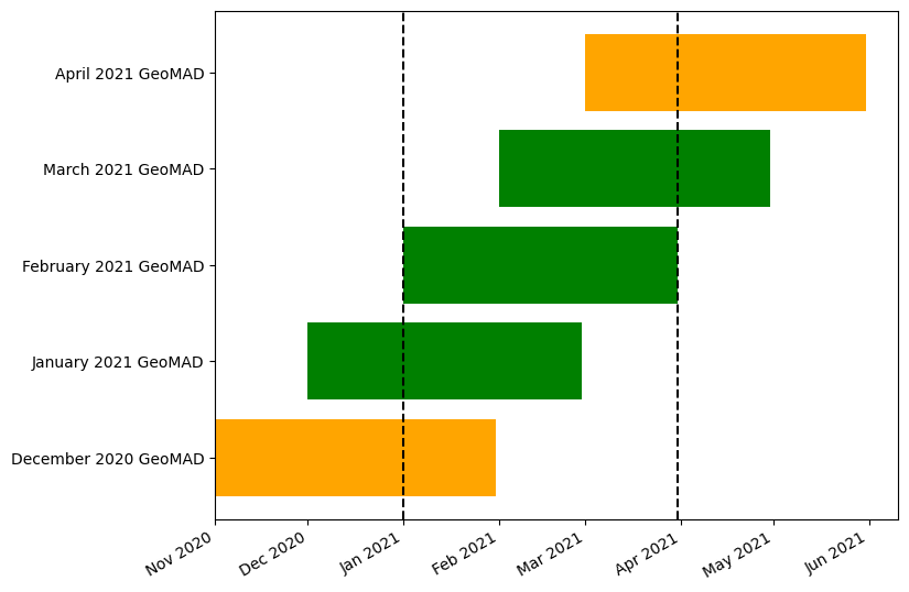
La nature évolutive de ce produit signifie que le comportement de chargement pour des périodes de temps spécifiées est différent des autres produits Digital Earth Africa. La raison en est qu’il existe un chevauchement temporel entre les images. Ceci est illustré ci-dessous dans le graphique qui conceptualise le comportement de chargement pour la période spécifiée « 2021-01-01 - 2021-03-31 » indiquée par des lignes noires en pointillés. Comme cette période couvre trois mois (janvier, février et mars), les utilisateurs peuvent s’attendre à ce que la requête renvoie trois images. Cependant, dans le cas du GeoMAD évolutif, cela renverra cinq images comme indiqué ci-dessous. C’est parce que la fonction « dc.load » importera toutes les images qui incluent des acquisitions d’images dans la période d’intérêt. Par exemple, le GeoMAD de décembre 2020 comprend des images de novembre et décembre 2020, et de janvier 2021, et sera donc chargé dans le cadre de la requête « 2021-01-01 - 2021-03-31 ». L’étiquette de date dans l’ensemble de données chargé sera « 2020-12-16 ».

begin = np.array(["2020-11-01", "2020-12-01", "2021-01-01", "2021-02-01", "2021-03-01"])
end =   np.array(["2021-01-31", "2021-02-28", "2021-03-31", "2021-04-30", "2021-05-31"])

begin = [datetime.strptime(i, "%Y-%m-%d") for i in begin]
end = [datetime.strptime(i, "%Y-%m-%d") for i in end]

event = ["December 2020 GeoMAD", "January 2021 GeoMAD", "February 2021 GeoMAD", "March 2021 GeoMAD", "April 2021 GeoMAD"]

fig, ax = plt.subplots(figsize=(8,6))

plt.barh(range(len(begin)),  [(end[i]-begin[i]) for i in range(len(begin))],
         left=begin, color=['orange', 'green', 'green', 'green', 'orange'])

plt.yticks(range(len(begin)), event)
ax.xaxis.set_major_locator(mdates.MonthLocator(interval=1))
ax.xaxis.set_major_formatter(mdates.DateFormatter("%b %Y"))
plt.setp(ax.get_xticklabels(), rotation=30, ha="right")
ax.axvline(x=datetime.strptime("2021-01-01", "%Y-%m-%d"), linestyle='dashed', color='black')
ax.axvline(x=datetime.strptime("2021-03-31", "%Y-%m-%d"), linestyle='dashed', color='black')
plt.show()

Le comportement de chargement décrit ci-dessus est évident dans le « ds » renvoyé ci-dessous.

ds = dc.load(product="gm_s2_rolling",
             measurements=['red','green','blue','nir','emad', 'smad', 'bcmad'],
             x=lon_range,
             y=lat_range,
             resolution=(-20, 20),
             output_crs = 'epsg:6933',
             time=("2021-01","2021-12"),

             )
display(ds)

<xarray.Dataset> Size: 29MB
Dimensions:      (time: 14, y: 359, x: 291)
Coordinates:
  * time         (time) datetime64[ns] 112B 2020-12-16T23:59:59.999999 ... 20...
  * y            (y) float64 3kB -2.626e+06 -2.626e+06 ... -2.633e+06 -2.633e+06
  * x            (x) float64 2kB 3.039e+06 3.039e+06 ... 3.045e+06 3.045e+06
    spatial_ref  int32 4B 6933
Data variables:
    red          (time, y, x) uint16 3MB 595 573 543 851 ... 1027 983 779 648
    green        (time, y, x) uint16 3MB 712 698 656 872 ... 1061 1026 929 886
    blue         (time, y, x) uint16 3MB 458 452 421 538 468 ... 728 704 638 597
    nir          (time, y, x) uint16 3MB 2634 2607 2514 2949 ... 3712 3597 3663
    emad         (time, y, x) float32 6MB 1.858e+03 1.863e+03 ... 1.197e+03
    smad         (time, y, x) float32 6MB 0.02137 0.01984 ... 0.001466 0.002157
    bcmad        (time, y, x) float32 6MB 0.1483 0.1527 ... 0.07304 0.07646
Attributes:
    crs:           epsg:6933
    grid_mapping:  spatial_ref

xarray.Dataset

• Dimensions:
  • time: 14
  • y: 359
  • x: 291
• Coordinates: (4)
  • time
    (time)
    datetime64[ns]
    2020-12-16T23:59:59.999999 ... 2...

    units :

    seconds since 1970-01-01 00:00:00

    array(['2020-12-16T23:59:59.999999000', '2021-01-14T23:59:59.999999000',
           '2021-02-14T23:59:59.999999000', '2021-03-17T11:59:59.999999000',
           '2021-04-15T23:59:59.999999000', '2021-05-16T11:59:59.999999000',
           '2021-06-15T23:59:59.999999000', '2021-07-16T23:59:59.999999000',
           '2021-08-15T23:59:59.999999000', '2021-09-15T23:59:59.999999000',
           '2021-10-16T11:59:59.999999000', '2021-11-15T23:59:59.999999000',
           '2021-12-16T23:59:59.999999000', '2022-01-14T23:59:59.999999000'],
          dtype='datetime64[ns]')

  • y
    (y)
    float64
    -2.626e+06 ... -2.633e+06

    units :

    metre

    resolution :

    -20.0

    crs :

    epsg:6933

    array([-2625730., -2625750., -2625770., ..., -2632850., -2632870., -2632890.])

  • x
    (x)
    float64
    3.039e+06 3.039e+06 ... 3.045e+06

    units :

    metre

    resolution :

    20.0

    crs :

    epsg:6933

    array([3039310., 3039330., 3039350., ..., 3045070., 3045090., 3045110.])

  • spatial_ref
    ()
    int32
    6933

    spatial_ref :

    PROJCS["WGS 84 / NSIDC EASE-Grid 2.0 Global",GEOGCS["WGS 84",DATUM["WGS_1984",SPHEROID["WGS 84",6378137,298.257223563,AUTHORITY["EPSG","7030"]],AUTHORITY["EPSG","6326"]],PRIMEM["Greenwich",0,AUTHORITY["EPSG","8901"]],UNIT["degree",0.0174532925199433,AUTHORITY["EPSG","9122"]],AUTHORITY["EPSG","4326"]],PROJECTION["Cylindrical_Equal_Area"],PARAMETER["standard_parallel_1",30],PARAMETER["central_meridian",0],PARAMETER["false_easting",0],PARAMETER["false_northing",0],UNIT["metre",1,AUTHORITY["EPSG","9001"]],AXIS["Easting",EAST],AXIS["Northing",NORTH],AUTHORITY["EPSG","6933"]]

    grid_mapping_name :

    lambert_cylindrical_equal_area

    array(6933, dtype=int32)

• Data variables: (7)
  • red
    (time, y, x)
    uint16
    595 573 543 851 ... 983 779 648

    units :

    1

    nodata :

    0

    crs :

    epsg:6933

    grid_mapping :

    spatial_ref

    array([[[ 595,  573,  543, ...,  657,  748,  794],
            [ 584,  554,  479, ...,  513,  686,  823],
            [ 544,  502,  438, ...,  475,  554,  747],
            ...,
            [1134, 1038,  902, ...,  514,  590,  593],
            [1250, 1249,  908, ...,  720,  601,  573],
            [1201, 1281,  857, ...,  898,  742,  586]],
    
           [[ 332,  336,  339, ...,  542,  574,  544],
            [ 323,  312,  320, ...,  448,  572,  580],
            [ 305,  289,  313, ...,  409,  485,  560],
            ...,
            [ 914,  734,  597, ...,  490,  520,  527],
            [1135,  986,  624, ...,  654,  522,  488],
            [1030, 1040,  563, ...,  807,  678,  493]],
    
           [[ 346,  348,  363, ...,  562,  553,  452],
            [ 332,  335,  336, ...,  434,  530,  479],
            [ 314,  323,  333, ...,  399,  458,  493],
            ...,
    ...
            ...,
            [1156, 1013,  928, ...,  647,  665,  638],
            [1241, 1216,  938, ...,  817,  685,  644],
            [1199, 1273,  883, ..., 1028,  841,  678]],
    
           [[ 497,  571,  570, ...,  811,  926, 1055],
            [ 502,  526,  481, ...,  624,  787, 1067],
            [ 482,  483,  440, ...,  556,  599,  905],
            ...,
            [1065,  905,  794, ...,  577,  568,  576],
            [1199, 1119,  789, ...,  767,  614,  598],
            [1145, 1215,  740, ..., 1007,  802,  636]],
    
           [[ 436,  473,  481, ...,  882,  830,  689],
            [ 423,  437,  423, ...,  661,  727,  718],
            [ 403,  413,  411, ...,  540,  582,  690],
            ...,
            [ 926,  687,  578, ...,  552,  508,  550],
            [1072,  967,  597, ...,  754,  575,  592],
            [ 993, 1089,  556, ...,  983,  779,  648]]], dtype=uint16)

  • green
    (time, y, x)
    uint16
    712 698 656 872 ... 1026 929 886

    units :

    1

    nodata :

    0

    crs :

    epsg:6933

    grid_mapping :

    spatial_ref

    array([[[ 712,  698,  656, ...,  705,  701,  740],
            [ 688,  660,  627, ...,  753,  741,  755],
            [ 669,  648,  639, ...,  767,  761,  751],
            ...,
            [ 900,  893,  846, ...,  774,  828,  827],
            [ 890,  961,  865, ...,  838,  821,  812],
            [ 881,  946,  828, ...,  910,  863,  801]],
    
           [[ 583,  602,  557, ...,  725,  706,  746],
            [ 578,  542,  542, ...,  739,  726,  748],
            [ 552,  525,  553, ...,  724,  744,  740],
            ...,
            [ 816,  736,  711, ...,  784,  802,  814],
            [ 838,  812,  725, ...,  819,  777,  772],
            [ 803,  813,  681, ...,  870,  819,  746]],
    
           [[ 571,  590,  568, ...,  740,  699,  718],
            [ 565,  549,  528, ...,  728,  717,  725],
            [ 531,  537,  537, ...,  710,  736,  727],
            ...,
    ...
            ...,
            [ 904,  886,  854, ...,  852,  859,  845],
            [ 920,  949,  867, ...,  901,  858,  846],
            [ 907,  949,  838, ...,  965,  904,  860]],
    
           [[ 696,  718,  676, ...,  752,  818,  878],
            [ 682,  661,  643, ...,  818,  832,  918],
            [ 659,  642,  650, ...,  814,  827,  883],
            ...,
            [ 889,  882,  831, ...,  824,  796,  806],
            [ 917,  938,  854, ...,  897,  825,  823],
            [ 911,  953,  838, ...,  983,  900,  838]],
    
           [[ 680,  704,  681, ...,  777,  786,  845],
            [ 665,  645,  639, ...,  871,  840,  856],
            [ 637,  632,  663, ...,  801,  839,  836],
            ...,
            [ 854,  831,  768, ...,  848,  770,  813],
            [ 862,  916,  820, ...,  941,  830,  861],
            [ 858,  923,  799, ..., 1026,  929,  886]]], dtype=uint16)

  • blue
    (time, y, x)
    uint16
    458 452 421 538 ... 728 704 638 597

    units :

    1

    nodata :

    0

    crs :

    epsg:6933

    grid_mapping :

    spatial_ref

    array([[[458, 452, 421, ..., 409, 422, 461],
            [454, 445, 390, ..., 446, 455, 472],
            [437, 423, 382, ..., 459, 454, 470],
            ...,
            [596, 585, 552, ..., 465, 522, 518],
            [608, 633, 564, ..., 522, 525, 510],
            [588, 621, 546, ..., 580, 554, 498]],
    
           [[317, 332, 320, ..., 388, 397, 442],
            [317, 311, 307, ..., 425, 424, 436],
            [302, 292, 302, ..., 416, 431, 434],
            ...,
            [510, 453, 435, ..., 474, 493, 492],
            [547, 512, 438, ..., 516, 475, 469],
            [506, 508, 424, ..., 545, 503, 446]],
    
           [[341, 353, 356, ..., 406, 396, 419],
            [333, 342, 335, ..., 414, 418, 426],
            [311, 335, 323, ..., 407, 428, 427],
            ...,
    ...
            ...,
            [674, 642, 602, ..., 580, 586, 576],
            [690, 688, 628, ..., 615, 593, 582],
            [676, 683, 614, ..., 660, 627, 591]],
    
           [[429, 484, 476, ..., 529, 578, 631],
            [437, 453, 432, ..., 556, 566, 663],
            [419, 428, 404, ..., 549, 539, 616],
            ...,
            [645, 629, 580, ..., 549, 519, 536],
            [676, 666, 593, ..., 618, 568, 554],
            [658, 670, 589, ..., 678, 622, 561]],
    
           [[406, 439, 452, ..., 529, 525, 554],
            [398, 416, 421, ..., 594, 556, 560],
            [383, 400, 411, ..., 527, 547, 545],
            ...,
            [580, 525, 473, ..., 566, 496, 538],
            [604, 591, 492, ..., 647, 568, 577],
            [582, 605, 483, ..., 704, 638, 597]]], dtype=uint16)

  • nir
    (time, y, x)
    uint16
    2634 2607 2514 ... 3712 3597 3663

    units :

    1

    nodata :

    0

    crs :

    epsg:6933

    grid_mapping :

    spatial_ref

    array([[[2634, 2607, 2514, ..., 2740, 2336, 2428],
            [2538, 2478, 2627, ..., 3650, 2723, 2331],
            [2553, 2540, 2898, ..., 3935, 3287, 2453],
            ...,
            [2109, 2410, 2511, ..., 3456, 3434, 3389],
            [2022, 2335, 2523, ..., 3339, 3382, 3397],
            [2165, 2282, 2417, ..., 3297, 3268, 3331]],
    
           [[3159, 3204, 2827, ..., 3086, 2823, 3159],
            [3092, 2946, 2923, ..., 4017, 3063, 2982],
            [2971, 2896, 3115, ..., 4262, 3596, 2999],
            ...,
            [2348, 2570, 2855, ..., 3666, 3628, 3649],
            [2239, 2444, 2810, ..., 3427, 3480, 3575],
            [2396, 2355, 2737, ..., 3340, 3300, 3444]],
    
           [[3047, 3147, 2828, ..., 3145, 2880, 3570],
            [2997, 2897, 2756, ..., 4085, 3204, 3353],
            [2863, 2795, 2943, ..., 4308, 3811, 3253],
            ...,
    ...
            ...,
            [2027, 2246, 2253, ..., 3291, 3201, 3212],
            [1998, 2211, 2291, ..., 3199, 3203, 3232],
            [2094, 2170, 2216, ..., 3216, 3178, 3225]],
    
           [[2967, 2635, 2467, ..., 2693, 2491, 2304],
            [2801, 2507, 2695, ..., 3580, 2849, 2387],
            [2753, 2601, 3066, ..., 3648, 3446, 2609],
            ...,
            [2276, 2591, 2599, ..., 3483, 3297, 3310],
            [2191, 2527, 2733, ..., 3356, 3310, 3339],
            [2412, 2464, 2683, ..., 3392, 3313, 3353]],
    
           [[3260, 3198, 3018, ..., 2777, 2825, 3278],
            [3185, 3019, 3206, ..., 3906, 3369, 3186],
            [3128, 3096, 3518, ..., 3946, 3852, 3149],
            ...,
            [2541, 3266, 3230, ..., 3836, 3482, 3510],
            [2415, 2985, 3390, ..., 3718, 3545, 3607],
            [2786, 2879, 3326, ..., 3712, 3597, 3663]]], dtype=uint16)

  • emad
    (time, y, x)
    float32
    1.858e+03 1.863e+03 ... 1.197e+03

    units :

    1

    nodata :

    nan

    crs :

    epsg:6933

    grid_mapping :

    spatial_ref

    array([[[1857.6212 , 1863.3562 , 1680.6012 , ..., 1066.8179 ,
             1272.2943 , 1708.4843 ],
            [1777.6759 , 1709.7549 , 1579.7837 , ..., 1108.06   ,
             1156.3281 , 1615.2346 ],
            [1843.8865 , 1601.3295 , 1242.5066 , ..., 1102.7524 ,
             1222.9237 , 1576.3911 ],
            ...,
            [1117.8892 , 1380.1302 , 1610.9783 , ...,  926.0729 ,
             1016.40894, 1018.16144],
            [ 930.322  , 1062.3909 , 1578.9326 , ...,  855.7098 ,
              897.48987, 1004.4348 ],
            [ 954.9895 , 1066.3472 , 1584.0234 , ...,  817.729  ,
              815.0276 ,  948.0534 ]],
    
           [[ 883.4602 ,  698.0722 ,  756.0382 , ...,  681.9756 ,
              802.4978 , 1062.8506 ],
            [ 797.2936 ,  678.6949 ,  710.59924, ...,  613.0127 ,
              803.667  ,  989.053  ],
            [ 659.32837,  676.4629 ,  677.51404, ...,  546.9034 ,
              674.12897,  801.3814 ],
    ...
            [ 898.931  , 1100.2771 , 1149.5083 , ...,  661.96436,
              636.28876,  639.231  ],
            [ 794.71875,  980.44336, 1141.0378 , ...,  749.71655,
              656.583  ,  649.29724],
            [ 971.8207 ,  987.5395 , 1147.8262 , ...,  805.5536 ,
              725.07605,  679.817  ]],
    
           [[ 745.7156 ,  998.0995 ,  944.79944, ...,  909.6976 ,
             1016.5341 , 1437.1604 ],
            [ 756.1997 ,  944.4486 ,  955.96313, ...,  826.12946,
             1037.8364 , 1636.5488 ],
            [ 856.0827 ,  862.62024, 1022.24695, ..., 1055.251  ,
              780.89087, 1339.8113 ],
            ...,
            [ 703.04846, 1206.2041 , 1467.554  , ..., 1112.5425 ,
             1235.4148 , 1362.1791 ],
            [ 725.24554,  914.3037 , 1302.5525 , ..., 1075.6918 ,
             1241.2236 , 1286.9438 ],
            [ 837.14484,  872.9153 , 1353.9728 , ...,  868.61316,
             1148.509  , 1196.6931 ]]], dtype=float32)

  • smad
    (time, y, x)
    float32
    0.02137 0.01984 ... 0.002157

    units :

    1

    nodata :

    nan

    crs :

    epsg:6933

    grid_mapping :

    spatial_ref

    array([[[0.02136888, 0.01984132, 0.01641147, ..., 0.00776155,
             0.01196958, 0.02056636],
            [0.02198221, 0.01922812, 0.01217688, ..., 0.00256106,
             0.00597131, 0.01932443],
            [0.01779023, 0.01385854, 0.00766251, ..., 0.00109396,
             0.00295413, 0.01367806],
            ...,
            [0.00981445, 0.01322931, 0.01983942, ..., 0.00161783,
             0.00291061, 0.00331894],
            [0.00584269, 0.00700087, 0.01711734, ..., 0.00177301,
             0.002427  , 0.00281792],
            [0.00846355, 0.00723816, 0.01976461, ..., 0.00193872,
             0.00209468, 0.00192782]],
    
           [[0.00043193, 0.00045521, 0.00102375, ..., 0.00134598,
             0.0017675 , 0.00280421],
            [0.00037763, 0.00048626, 0.00093044, ..., 0.00076761,
             0.00113577, 0.00256659],
            [0.00039096, 0.00045991, 0.00071193, ..., 0.00024445,
             0.00047689, 0.001492  ],
    ...
            [0.00787011, 0.01270821, 0.01241999, ..., 0.00212154,
             0.00258931, 0.00243263],
            [0.00625508, 0.00654496, 0.01221419, ..., 0.00189609,
             0.00212202, 0.00245512],
            [0.00604361, 0.00489699, 0.01268377, ..., 0.00225395,
             0.00178401, 0.00277092]],
    
           [[0.00110101, 0.00105915, 0.00106003, ..., 0.0014778 ,
             0.00242894, 0.00169154],
            [0.00099574, 0.00092789, 0.0008066 , ..., 0.00078247,
             0.00164571, 0.00198787],
            [0.00085703, 0.00070497, 0.00072196, ..., 0.00076839,
             0.00086591, 0.00167272],
            ...,
            [0.00229941, 0.0020972 , 0.00216098, ..., 0.00136152,
             0.00154885, 0.00155924],
            [0.00161681, 0.00194409, 0.00114526, ..., 0.0010843 ,
             0.0013867 , 0.00198877],
            [0.0027595 , 0.00171854, 0.00111168, ..., 0.00096073,
             0.00146599, 0.00215656]]], dtype=float32)

  • bcmad
    (time, y, x)
    float32
    0.1483 0.1527 ... 0.07304 0.07646

    units :

    1

    nodata :

    nan

    crs :

    epsg:6933

    grid_mapping :

    spatial_ref

    array([[[0.14828521, 0.15272874, 0.1337116 , ..., 0.08098768,
             0.0977214 , 0.12283759],
            [0.14984831, 0.14341891, 0.12582216, ..., 0.06862941,
             0.08406644, 0.12305154],
            [0.15710732, 0.13482723, 0.09458651, ..., 0.05848889,
             0.0721702 , 0.11186589],
            ...,
            [0.07985804, 0.10419788, 0.13200198, ..., 0.06110061,
             0.07239856, 0.07521698],
            [0.06339842, 0.0775835 , 0.11821406, ..., 0.05488772,
             0.05808758, 0.07166536],
            [0.06835334, 0.07460007, 0.11133011, ..., 0.05031081,
             0.05180496, 0.06100992]],
    
           [[0.06660194, 0.05509581, 0.05761881, ..., 0.04513965,
             0.05807946, 0.07383181],
            [0.06212482, 0.05460145, 0.05292827, ..., 0.03404583,
             0.05485335, 0.07628732],
            [0.05460042, 0.05279858, 0.05037886, ..., 0.03244693,
             0.03962108, 0.06293181],
    ...
            [0.06874567, 0.08579738, 0.09760857, ..., 0.04780991,
             0.04632411, 0.04798122],
            [0.05886952, 0.07298692, 0.08990717, ..., 0.05268919,
             0.04826033, 0.04758994],
            [0.06923564, 0.06912291, 0.09358017, ..., 0.05682427,
             0.05420631, 0.04862339]],
    
           [[0.05162803, 0.08180498, 0.07378963, ..., 0.07242478,
             0.07082845, 0.08508941],
            [0.05389614, 0.0795915 , 0.07476562, ..., 0.05432424,
             0.07207082, 0.09868196],
            [0.05933953, 0.06901819, 0.0764294 , ..., 0.05243541,
             0.0479064 , 0.08364818],
            ...,
            [0.05518123, 0.08111189, 0.08902945, ..., 0.06920368,
             0.07957728, 0.08392631],
            [0.05273411, 0.06703328, 0.07454018, ..., 0.0638847 ,
             0.07999644, 0.08027983],
            [0.0529424 , 0.06037455, 0.08811028, ..., 0.04840375,
             0.0730436 , 0.07645582]]], dtype=float32)

• Indexes: (3)
  • time
    PandasIndex

    PandasIndex(DatetimeIndex(['2020-12-16 23:59:59.999999', '2021-01-14 23:59:59.999999',
                   '2021-02-14 23:59:59.999999', '2021-03-17 11:59:59.999999',
                   '2021-04-15 23:59:59.999999', '2021-05-16 11:59:59.999999',
                   '2021-06-15 23:59:59.999999', '2021-07-16 23:59:59.999999',
                   '2021-08-15 23:59:59.999999', '2021-09-15 23:59:59.999999',
                   '2021-10-16 11:59:59.999999', '2021-11-15 23:59:59.999999',
                   '2021-12-16 23:59:59.999999', '2022-01-14 23:59:59.999999'],
                  dtype='datetime64[ns]', name='time', freq=None))

  • y
    PandasIndex

    PandasIndex(Index([-2625730.0, -2625750.0, -2625770.0, -2625790.0, -2625810.0, -2625830.0,
           -2625850.0, -2625870.0, -2625890.0, -2625910.0,
           ...
           -2632710.0, -2632730.0, -2632750.0, -2632770.0, -2632790.0, -2632810.0,
           -2632830.0, -2632850.0, -2632870.0, -2632890.0],
          dtype='float64', name='y', length=359))

  • x
    PandasIndex

    PandasIndex(Index([3039310.0, 3039330.0, 3039350.0, 3039370.0, 3039390.0, 3039410.0,
           3039430.0, 3039450.0, 3039470.0, 3039490.0,
           ...
           3044930.0, 3044950.0, 3044970.0, 3044990.0, 3045010.0, 3045030.0,
           3045050.0, 3045070.0, 3045090.0, 3045110.0],
          dtype='float64', name='x', length=291))

• Attributes: (2)

  crs :

  epsg:6933

  grid_mapping :

  spatial_ref

La cellule ci-dessous découpe les heures de début et de fin pour obtenir la plage horaire spécifiée. Notez que l’objet « ds » ci-dessous inclut uniquement les images étiquetées « 2021 ».

ds_time = ds.time[1:-1]
ds = ds.sel(time=ds_time.values)
display(ds)

<xarray.Dataset> Size: 25MB
Dimensions:      (time: 12, y: 359, x: 291)
Coordinates:
  * time         (time) datetime64[ns] 96B 2021-01-14T23:59:59.999999 ... 202...
  * y            (y) float64 3kB -2.626e+06 -2.626e+06 ... -2.633e+06 -2.633e+06
  * x            (x) float64 2kB 3.039e+06 3.039e+06 ... 3.045e+06 3.045e+06
    spatial_ref  int32 4B 6933
Data variables:
    red          (time, y, x) uint16 3MB 332 336 339 678 ... 1053 1007 802 636
    green        (time, y, x) uint16 3MB 583 602 557 781 ... 1027 983 900 838
    blue         (time, y, x) uint16 3MB 317 332 320 451 376 ... 704 678 622 561
    nir          (time, y, x) uint16 3MB 3159 3204 2827 3226 ... 3392 3313 3353
    emad         (time, y, x) float32 5MB 883.5 698.1 756.0 ... 725.1 679.8
    smad         (time, y, x) float32 5MB 0.0004319 0.0004552 ... 0.002771
    bcmad        (time, y, x) float32 5MB 0.0666 0.0551 ... 0.05421 0.04862
Attributes:
    crs:           epsg:6933
    grid_mapping:  spatial_ref

xarray.Dataset

• Dimensions:
  • time: 12
  • y: 359
  • x: 291
• Coordinates: (4)
  • time
    (time)
    datetime64[ns]
    2021-01-14T23:59:59.999999 ... 2...

    units :

    seconds since 1970-01-01 00:00:00

    array(['2021-01-14T23:59:59.999999000', '2021-02-14T23:59:59.999999000',
           '2021-03-17T11:59:59.999999000', '2021-04-15T23:59:59.999999000',
           '2021-05-16T11:59:59.999999000', '2021-06-15T23:59:59.999999000',
           '2021-07-16T23:59:59.999999000', '2021-08-15T23:59:59.999999000',
           '2021-09-15T23:59:59.999999000', '2021-10-16T11:59:59.999999000',
           '2021-11-15T23:59:59.999999000', '2021-12-16T23:59:59.999999000'],
          dtype='datetime64[ns]')

  • y
    (y)
    float64
    -2.626e+06 ... -2.633e+06

    units :

    metre

    resolution :

    -20.0

    crs :

    epsg:6933

    array([-2625730., -2625750., -2625770., ..., -2632850., -2632870., -2632890.])

  • x
    (x)
    float64
    3.039e+06 3.039e+06 ... 3.045e+06

    units :

    metre

    resolution :

    20.0

    crs :

    epsg:6933

    array([3039310., 3039330., 3039350., ..., 3045070., 3045090., 3045110.])

  • spatial_ref
    ()
    int32
    6933

    spatial_ref :

    PROJCS["WGS 84 / NSIDC EASE-Grid 2.0 Global",GEOGCS["WGS 84",DATUM["WGS_1984",SPHEROID["WGS 84",6378137,298.257223563,AUTHORITY["EPSG","7030"]],AUTHORITY["EPSG","6326"]],PRIMEM["Greenwich",0,AUTHORITY["EPSG","8901"]],UNIT["degree",0.0174532925199433,AUTHORITY["EPSG","9122"]],AUTHORITY["EPSG","4326"]],PROJECTION["Cylindrical_Equal_Area"],PARAMETER["standard_parallel_1",30],PARAMETER["central_meridian",0],PARAMETER["false_easting",0],PARAMETER["false_northing",0],UNIT["metre",1,AUTHORITY["EPSG","9001"]],AXIS["Easting",EAST],AXIS["Northing",NORTH],AUTHORITY["EPSG","6933"]]

    grid_mapping_name :

    lambert_cylindrical_equal_area

    array(6933, dtype=int32)

• Data variables: (7)
  • red
    (time, y, x)
    uint16
    332 336 339 678 ... 1007 802 636

    units :

    1

    nodata :

    0

    crs :

    epsg:6933

    grid_mapping :

    spatial_ref

    array([[[ 332,  336,  339, ...,  542,  574,  544],
            [ 323,  312,  320, ...,  448,  572,  580],
            [ 305,  289,  313, ...,  409,  485,  560],
            ...,
            [ 914,  734,  597, ...,  490,  520,  527],
            [1135,  986,  624, ...,  654,  522,  488],
            [1030, 1040,  563, ...,  807,  678,  493]],
    
           [[ 346,  348,  363, ...,  562,  553,  452],
            [ 332,  335,  336, ...,  434,  530,  479],
            [ 314,  323,  333, ...,  399,  458,  493],
            ...,
            [ 859,  752,  552, ...,  468,  489,  496],
            [1035,  996,  576, ...,  612,  504,  475],
            [ 944, 1082,  548, ...,  782,  638,  495]],
    
           [[ 418,  439,  445, ...,  648,  586,  441],
            [ 411,  424,  395, ...,  431,  526,  461],
            [ 400,  419,  387, ...,  404,  450,  482],
            ...,
    ...
            ...,
            [1135, 1050,  982, ...,  774,  797,  751],
            [1208, 1249,  983, ..., 1000,  832,  774],
            [1131, 1298,  954, ..., 1109,  965,  825]],
    
           [[ 796,  813,  771, ...,  724,  879, 1079],
            [ 801,  753,  661, ...,  611,  767, 1059],
            [ 780,  706,  612, ...,  601,  637,  916],
            ...,
            [1156, 1013,  928, ...,  647,  665,  638],
            [1241, 1216,  938, ...,  817,  685,  644],
            [1199, 1273,  883, ..., 1028,  841,  678]],
    
           [[ 497,  571,  570, ...,  811,  926, 1055],
            [ 502,  526,  481, ...,  624,  787, 1067],
            [ 482,  483,  440, ...,  556,  599,  905],
            ...,
            [1065,  905,  794, ...,  577,  568,  576],
            [1199, 1119,  789, ...,  767,  614,  598],
            [1145, 1215,  740, ..., 1007,  802,  636]]], dtype=uint16)

  • green
    (time, y, x)
    uint16
    583 602 557 781 ... 983 900 838

    units :

    1

    nodata :

    0

    crs :

    epsg:6933

    grid_mapping :

    spatial_ref

    array([[[583, 602, 557, ..., 725, 706, 746],
            [578, 542, 542, ..., 739, 726, 748],
            [552, 525, 553, ..., 724, 744, 740],
            ...,
            [816, 736, 711, ..., 784, 802, 814],
            [838, 812, 725, ..., 819, 777, 772],
            [803, 813, 681, ..., 870, 819, 746]],
    
           [[571, 590, 568, ..., 740, 699, 718],
            [565, 549, 528, ..., 728, 717, 725],
            [531, 537, 537, ..., 710, 736, 727],
            ...,
            [839, 842, 785, ..., 773, 791, 807],
            [818, 870, 791, ..., 794, 775, 776],
            [805, 874, 769, ..., 851, 802, 752]],
    
           [[546, 564, 548, ..., 734, 675, 716],
            [554, 543, 512, ..., 713, 746, 726],
            [528, 529, 503, ..., 715, 752, 743],
            ...,
    ...
            ...,
            [923, 953, 944, ..., 798, 808, 802],
            [915, 980, 945, ..., 887, 819, 822],
            [882, 976, 938, ..., 930, 868, 829]],
    
           [[763, 763, 741, ..., 748, 822, 927],
            [756, 728, 712, ..., 818, 838, 952],
            [736, 704, 726, ..., 851, 847, 908],
            ...,
            [904, 886, 854, ..., 852, 859, 845],
            [920, 949, 867, ..., 901, 858, 846],
            [907, 949, 838, ..., 965, 904, 860]],
    
           [[696, 718, 676, ..., 752, 818, 878],
            [682, 661, 643, ..., 818, 832, 918],
            [659, 642, 650, ..., 814, 827, 883],
            ...,
            [889, 882, 831, ..., 824, 796, 806],
            [917, 938, 854, ..., 897, 825, 823],
            [911, 953, 838, ..., 983, 900, 838]]], dtype=uint16)

  • blue
    (time, y, x)
    uint16
    317 332 320 451 ... 704 678 622 561

    units :

    1

    nodata :

    0

    crs :

    epsg:6933

    grid_mapping :

    spatial_ref

    array([[[317, 332, 320, ..., 388, 397, 442],
            [317, 311, 307, ..., 425, 424, 436],
            [302, 292, 302, ..., 416, 431, 434],
            ...,
            [510, 453, 435, ..., 474, 493, 492],
            [547, 512, 438, ..., 516, 475, 469],
            [506, 508, 424, ..., 545, 503, 446]],
    
           [[341, 353, 356, ..., 406, 396, 419],
            [333, 342, 335, ..., 414, 418, 426],
            [311, 335, 323, ..., 407, 428, 427],
            ...,
            [513, 509, 443, ..., 462, 472, 468],
            [541, 548, 449, ..., 487, 459, 449],
            [521, 546, 447, ..., 521, 482, 434]],
    
           [[336, 356, 360, ..., 441, 409, 412],
            [331, 351, 327, ..., 407, 434, 420],
            [319, 335, 308, ..., 418, 442, 427],
            ...,
    ...
            ...,
            [675, 671, 662, ..., 578, 591, 594],
            [659, 692, 665, ..., 625, 593, 603],
            [626, 686, 661, ..., 638, 616, 605]],
    
           [[598, 617, 594, ..., 511, 573, 653],
            [602, 579, 543, ..., 563, 573, 676],
            [581, 558, 521, ..., 605, 577, 633],
            ...,
            [674, 642, 602, ..., 580, 586, 576],
            [690, 688, 628, ..., 615, 593, 582],
            [676, 683, 614, ..., 660, 627, 591]],
    
           [[429, 484, 476, ..., 529, 578, 631],
            [437, 453, 432, ..., 556, 566, 663],
            [419, 428, 404, ..., 549, 539, 616],
            ...,
            [645, 629, 580, ..., 549, 519, 536],
            [676, 666, 593, ..., 618, 568, 554],
            [658, 670, 589, ..., 678, 622, 561]]], dtype=uint16)

  • nir
    (time, y, x)
    uint16
    3159 3204 2827 ... 3392 3313 3353

    units :

    1

    nodata :

    0

    crs :

    epsg:6933

    grid_mapping :

    spatial_ref

    array([[[3159, 3204, 2827, ..., 3086, 2823, 3159],
            [3092, 2946, 2923, ..., 4017, 3063, 2982],
            [2971, 2896, 3115, ..., 4262, 3596, 2999],
            ...,
            [2348, 2570, 2855, ..., 3666, 3628, 3649],
            [2239, 2444, 2810, ..., 3427, 3480, 3575],
            [2396, 2355, 2737, ..., 3340, 3300, 3444]],
    
           [[3047, 3147, 2828, ..., 3145, 2880, 3570],
            [2997, 2897, 2756, ..., 4085, 3204, 3353],
            [2863, 2795, 2943, ..., 4308, 3811, 3253],
            ...,
            [2772, 3049, 3348, ..., 3971, 4038, 4053],
            [2446, 2713, 3240, ..., 3618, 3786, 3974],
            [2523, 2618, 3180, ..., 3441, 3540, 3819]],
    
           [[2563, 2643, 2430, ..., 3111, 2812, 3818],
            [2588, 2432, 2394, ..., 4426, 3756, 3602],
            [2551, 2360, 2494, ..., 4491, 4250, 3573],
            ...,
    ...
            ...,
            [2159, 2405, 2451, ..., 2393, 2339, 2339],
            [2067, 2268, 2425, ..., 2577, 2426, 2429],
            [2115, 2237, 2386, ..., 2693, 2500, 2418]],
    
           [[1937, 1807, 1815, ..., 2857, 2539, 2380],
            [1869, 1784, 2063, ..., 3408, 2726, 2438],
            [1857, 1828, 2463, ..., 3455, 3234, 2566],
            ...,
            [2027, 2246, 2253, ..., 3291, 3201, 3212],
            [1998, 2211, 2291, ..., 3199, 3203, 3232],
            [2094, 2170, 2216, ..., 3216, 3178, 3225]],
    
           [[2967, 2635, 2467, ..., 2693, 2491, 2304],
            [2801, 2507, 2695, ..., 3580, 2849, 2387],
            [2753, 2601, 3066, ..., 3648, 3446, 2609],
            ...,
            [2276, 2591, 2599, ..., 3483, 3297, 3310],
            [2191, 2527, 2733, ..., 3356, 3310, 3339],
            [2412, 2464, 2683, ..., 3392, 3313, 3353]]], dtype=uint16)

  • emad
    (time, y, x)
    float32
    883.5 698.1 756.0 ... 725.1 679.8

    units :

    1

    nodata :

    nan

    crs :

    epsg:6933

    grid_mapping :

    spatial_ref

    array([[[ 883.4602 ,  698.0722 ,  756.0382 , ...,  681.9756 ,
              802.4978 , 1062.8506 ],
            [ 797.2936 ,  678.6949 ,  710.59924, ...,  613.0127 ,
              803.667  ,  989.053  ],
            [ 659.32837,  676.4629 ,  677.51404, ...,  546.9034 ,
              674.12897,  801.3814 ],
            ...,
            [ 940.7304 ,  990.8058 , 1301.2698 , ...,  749.57825,
              856.1123 , 1220.1659 ],
            [ 786.5332 ,  953.4821 , 1313.8693 , ...,  787.4095 ,
              775.59766,  935.5133 ],
            [ 959.708  ,  896.88605, 1317.1594 , ...,  833.24384,
              778.1986 ,  756.0571 ]],
    
           [[ 710.34656,  700.86475,  688.9086 , ...,  744.4963 ,
              525.64636,  620.74713],
            [ 653.80084,  716.0927 ,  740.587  , ...,  762.611  ,
              917.2253 ,  620.88   ],
            [ 634.14154,  726.8873 ,  814.67   , ...,  687.87976,
              925.05066,  704.91156],
    ...
            [ 746.12476, 1034.6244 , 1075.6404 , ...,  844.04956,
              806.60706,  749.9962 ],
            [ 572.96967,  903.0728 , 1137.3718 , ...,  946.8973 ,
              881.4224 ,  773.77014],
            [ 738.29834,  843.6172 , 1139.5962 , ...,  999.0752 ,
              946.64813,  815.08575]],
    
           [[1301.4983 , 1390.3354 , 1548.5203 , ...,  852.14777,
              947.521  , 1311.6895 ],
            [1390.0593 , 1416.2764 , 1566.4202 , ...,  566.3817 ,
              682.2355 , 1129.782  ],
            [1545.4335 , 1601.5371 , 1360.3889 , ...,  816.7023 ,
              655.1493 ,  942.548  ],
            ...,
            [ 898.931  , 1100.2771 , 1149.5083 , ...,  661.96436,
              636.28876,  639.231  ],
            [ 794.71875,  980.44336, 1141.0378 , ...,  749.71655,
              656.583  ,  649.29724],
            [ 971.8207 ,  987.5395 , 1147.8262 , ...,  805.5536 ,
              725.07605,  679.817  ]]], dtype=float32)

  • smad
    (time, y, x)
    float32
    0.0004319 0.0004552 ... 0.002771

    units :

    1

    nodata :

    nan

    crs :

    epsg:6933

    grid_mapping :

    spatial_ref

    array([[[0.00043193, 0.00045521, 0.00102375, ..., 0.00134598,
             0.0017675 , 0.00280421],
            [0.00037763, 0.00048626, 0.00093044, ..., 0.00076761,
             0.00113577, 0.00256659],
            [0.00039096, 0.00045991, 0.00071193, ..., 0.00024445,
             0.00047689, 0.001492  ],
            ...,
            [0.00383902, 0.00830226, 0.00480975, ..., 0.00045246,
             0.00057815, 0.00080944],
            [0.00409419, 0.00782871, 0.00484323, ..., 0.00068543,
             0.00059567, 0.0006849 ],
            [0.00765281, 0.00573506, 0.00401132, ..., 0.00091917,
             0.00061745, 0.00064094]],
    
           [[0.00098348, 0.00102905, 0.00131521, ..., 0.00118137,
             0.00111193, 0.00083004],
            [0.00098959, 0.0012572 , 0.00166559, ..., 0.00065295,
             0.00112767, 0.0011965 ],
            [0.0010716 , 0.001241  , 0.00101069, ..., 0.00042097,
             0.00093473, 0.00110958],
    ...
            [0.00644078, 0.01094025, 0.01183491, ..., 0.00307548,
             0.0031878 , 0.00269544],
            [0.00391962, 0.00783384, 0.01141465, ..., 0.0029951 ,
             0.0031785 , 0.00264242],
            [0.00503181, 0.005667  , 0.01186462, ..., 0.00269398,
             0.00280442, 0.00274943]],
    
           [[0.00518559, 0.01042317, 0.00900707, ..., 0.00203089,
             0.0066672 , 0.01393587],
            [0.0061243 , 0.00906882, 0.00702715, ..., 0.00107615,
             0.00249086, 0.0104608 ],
            [0.0061104 , 0.00661683, 0.00376531, ..., 0.00091718,
             0.0007087 , 0.00627805],
            ...,
            [0.00787011, 0.01270821, 0.01241999, ..., 0.00212154,
             0.00258931, 0.00243263],
            [0.00625508, 0.00654496, 0.01221419, ..., 0.00189609,
             0.00212202, 0.00245512],
            [0.00604361, 0.00489699, 0.01268377, ..., 0.00225395,
             0.00178401, 0.00277092]]], dtype=float32)

  • bcmad
    (time, y, x)
    float32
    0.0666 0.0551 ... 0.05421 0.04862

    units :

    1

    nodata :

    nan

    crs :

    epsg:6933

    grid_mapping :

    spatial_ref

    array([[[0.06660194, 0.05509581, 0.05761881, ..., 0.04513965,
             0.05807946, 0.07383181],
            [0.06212482, 0.05460145, 0.05292827, ..., 0.03404583,
             0.05485335, 0.07628732],
            [0.05460042, 0.05279858, 0.05037886, ..., 0.03244693,
             0.03962108, 0.06293181],
            ...,
            [0.06505226, 0.07878131, 0.08941947, ..., 0.04798441,
             0.05861875, 0.0780866 ],
            [0.05889361, 0.07168985, 0.09214188, ..., 0.05253913,
             0.05227297, 0.06245357],
            [0.06560093, 0.06559402, 0.09293608, ..., 0.05611992,
             0.05191286, 0.05209284]],
    
           [[0.05559639, 0.05243459, 0.0543134 , ..., 0.0495369 ,
             0.04041103, 0.03837506],
            [0.05410305, 0.05492347, 0.05898091, ..., 0.03942092,
             0.06200912, 0.04630551],
            [0.0504673 , 0.0636262 , 0.06394364, ..., 0.03704562,
             0.06086303, 0.0498372 ],
    ...
            [0.05875989, 0.07817611, 0.08388828, ..., 0.05689482,
             0.05464803, 0.05120419],
            [0.04308672, 0.0704229 , 0.09544806, ..., 0.05730322,
             0.0551922 , 0.05196949],
            [0.05623114, 0.06412847, 0.09191526, ..., 0.05663468,
             0.05500218, 0.05303663]],
    
           [[0.08958156, 0.10196535, 0.11587732, ..., 0.06389952,
             0.07044461, 0.10075244],
            [0.0933533 , 0.11005333, 0.11667189, ..., 0.03682243,
             0.05233968, 0.08615816],
            [0.1001544 , 0.12637272, 0.10267639, ..., 0.05056223,
             0.04357365, 0.07224344],
            ...,
            [0.06874567, 0.08579738, 0.09760857, ..., 0.04780991,
             0.04632411, 0.04798122],
            [0.05886952, 0.07298692, 0.08990717, ..., 0.05268919,
             0.04826033, 0.04758994],
            [0.06923564, 0.06912291, 0.09358017, ..., 0.05682427,
             0.05420631, 0.04862339]]], dtype=float32)

• Indexes: (3)
  • time
    PandasIndex

    PandasIndex(DatetimeIndex(['2021-01-14 23:59:59.999999', '2021-02-14 23:59:59.999999',
                   '2021-03-17 11:59:59.999999', '2021-04-15 23:59:59.999999',
                   '2021-05-16 11:59:59.999999', '2021-06-15 23:59:59.999999',
                   '2021-07-16 23:59:59.999999', '2021-08-15 23:59:59.999999',
                   '2021-09-15 23:59:59.999999', '2021-10-16 11:59:59.999999',
                   '2021-11-15 23:59:59.999999', '2021-12-16 23:59:59.999999'],
                  dtype='datetime64[ns]', name='time', freq=None))

  • y
    PandasIndex

    PandasIndex(Index([-2625730.0, -2625750.0, -2625770.0, -2625790.0, -2625810.0, -2625830.0,
           -2625850.0, -2625870.0, -2625890.0, -2625910.0,
           ...
           -2632710.0, -2632730.0, -2632750.0, -2632770.0, -2632790.0, -2632810.0,
           -2632830.0, -2632850.0, -2632870.0, -2632890.0],
          dtype='float64', name='y', length=359))

  • x
    PandasIndex

    PandasIndex(Index([3039310.0, 3039330.0, 3039350.0, 3039370.0, 3039390.0, 3039410.0,
           3039430.0, 3039450.0, 3039470.0, 3039490.0,
           ...
           3044930.0, 3044950.0, 3044970.0, 3044990.0, 3045010.0, 3045030.0,
           3045050.0, 3045070.0, 3045090.0, 3045110.0],
          dtype='float64', name='x', length=291))

• Attributes: (2)

  crs :

  epsg:6933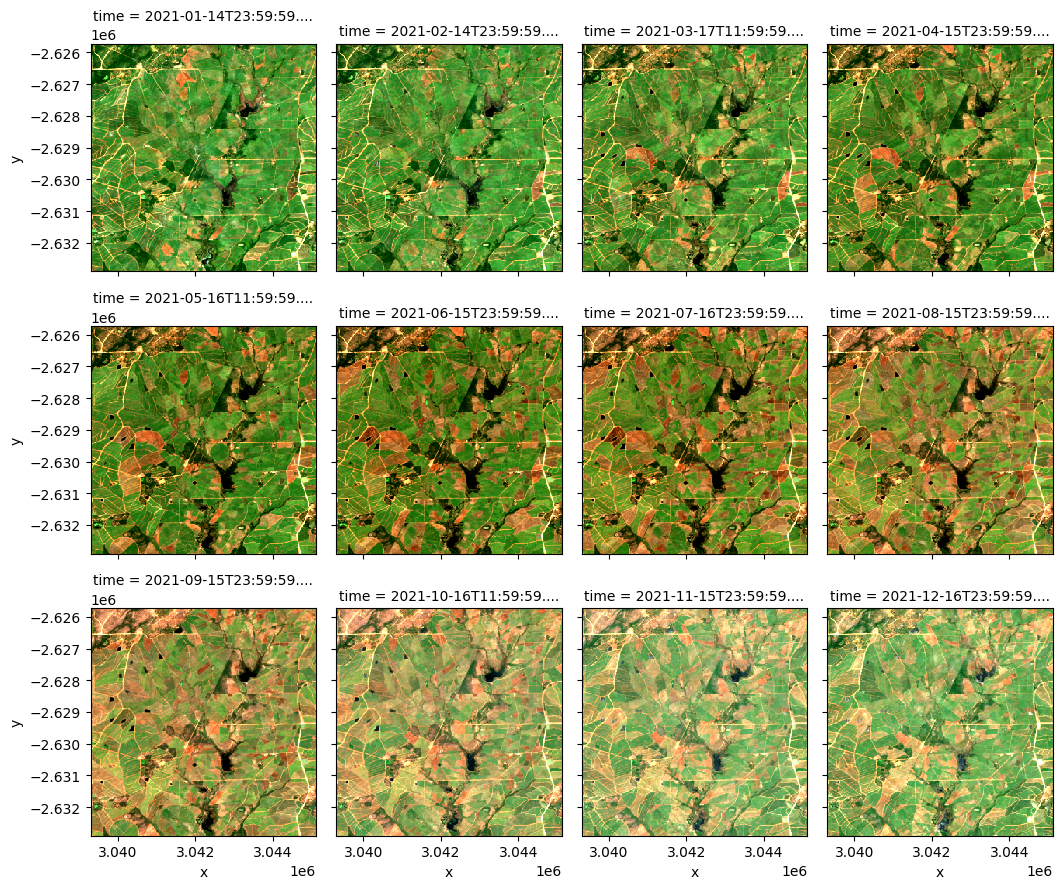

  grid_mapping :

  spatial_ref

Affichage RVB du Sentinel-2 Rolling GeoMAD

Nous pouvons tracer les données que nous avons chargées à l’aide de la fonction « rgb() ». Par défaut, la fonction tracera les données sous forme d’image en vraies couleurs à l’aide des bandes « rouge », « verte » et « bleue ».

rgb(ds, col='time', col_wrap=4, size=3)

Calculer le NDVI en utilisant « calculer les indices »

Reportez-vous au bloc-notes « Calcul des indices de bande <../Frequently_used_code/Calculating_band_indices.ipynb> » pour plus d’informations. >Remarque : ce produit convient au calcul de tous les indices, pas seulement du NDVI.

ds_NDVI = calculate_indices(ds, index=['NDVI'], satellite_mission='s2')

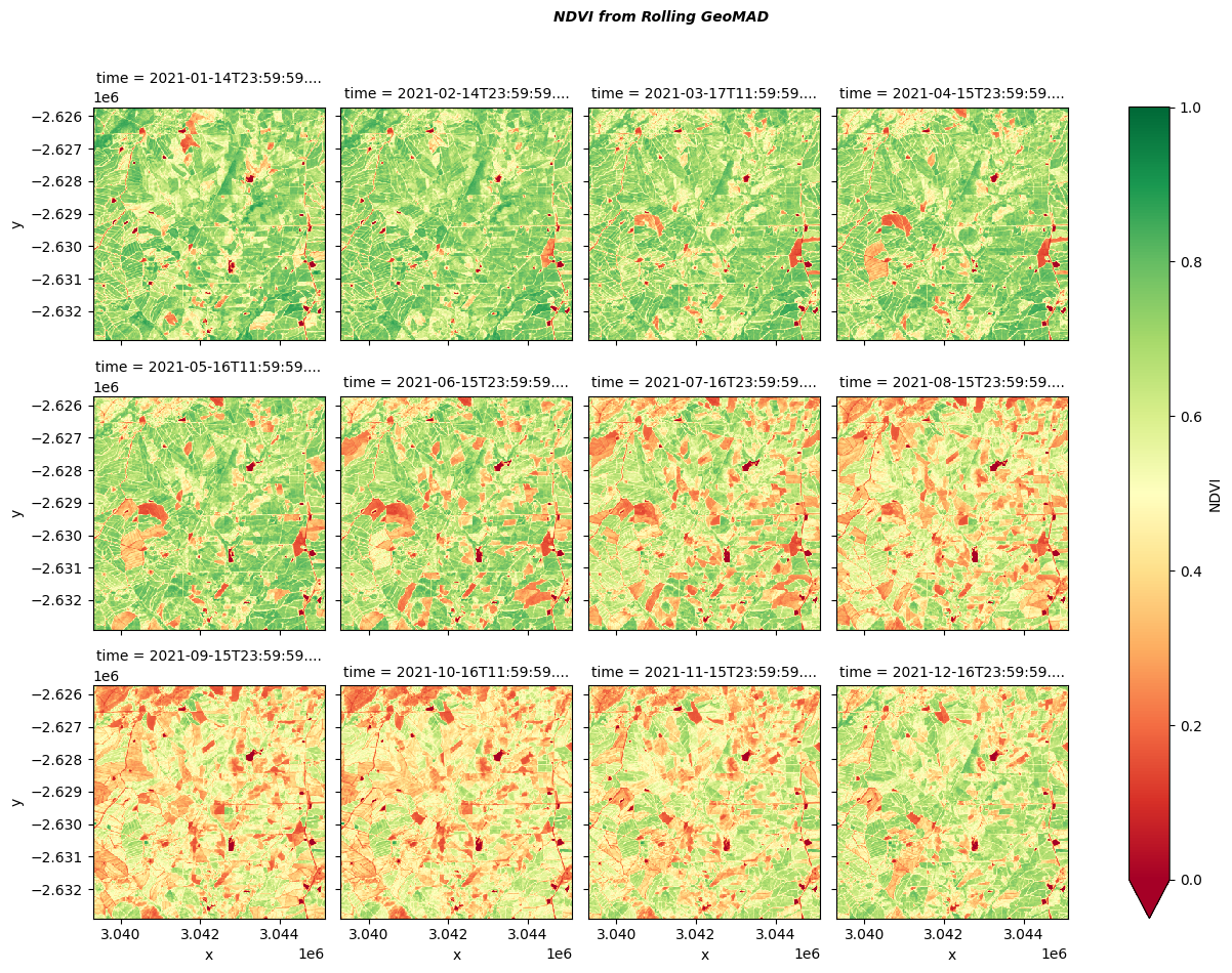
Graphique NDVI

Le NDVI est représenté ci-dessous pour chaque mois de 2021. Existe-t-il des tendances ou des changements notables dans la distribution du NDVI dans l’espace ?

# NDVI Rolling GeoMAD
ds_NDVI.NDVI.plot(x='x',y='y', col='time', col_wrap = 4, vmin=0, vmax=1,
                                           cmap='RdYlGn', robust=True)

# Title NDVI Rolling GeoMAD
plt.suptitle('NDVI from Rolling GeoMAD', y = 1.05, fontproperties={'style':'oblique', 'weight':'bold'})

plt.show()

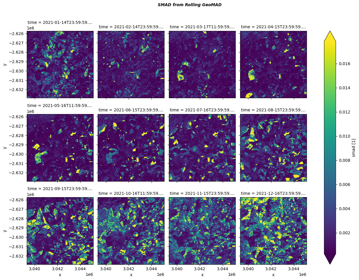
Terrain SMAD

Les bandes d’écart absolu médian (MAD) fournissent des informations sur les changements au cours de la période de calcul géomédiane. Cela se fait tout en préservant les relations à haute dimension entre les bandes satellites. Par exemple, des valeurs d’écart absolu médian spectral (SMAD) plus élevées indiquent une plus grande quantité de changement au cours d’une période ; dans ce cas, la fenêtre glissante de trois mois.

Ces informations peuvent aider à identifier les zones les plus dynamiques au cours d’une période donnée. Dans les environnements gérés (par exemple agricoles), cela peut concerner des activités telles que la culture, la récolte ou la plantation de cultures.

En examinant les images ci-dessous, pouvez-vous identifier les champs de la plantation de canne à sucre qui ont subi des changements ? Essayez de comparer ces champs avec les images NDVI et RVB ci-dessus pour voir si vous pouvez tirer des conclusions sur ce qui s’est passé.

ds.smad.plot(x='x',y='y', col='time', col_wrap=4, cmap='viridis', robust=True)

plt.suptitle('SMAD from Rolling GeoMAD', y = 1.05, fontproperties={'style':'oblique', 'weight':'bold'})

plt.show()

Conclusion

Ce carnet a démontré le chargement et le traçage du Rolling GeoMAD. Il a également montré comment la nature évolutive de ce produit signifie que ses images se chevauchent dans le temps, ce qui a des implications sur les procédures de chargement.

---

Informations Complémentaires

Licence : Le code de ce carnet est sous licence Apache, version 2.0 <https://www.apache.org/licenses/LICENSE-2.0>. Les données de Digital Earth Africa sont sous licence Creative Commons par attribution 4.0 <https://creativecommons.org/licenses/by/4.0/>.

Contact : Si vous avez besoin d’aide, veuillez poster une question sur le canal Slack Open Data Cube <http://slack.opendatacube.org/>`__ ou sur le GIS Stack Exchange en utilisant la balise open-data-cube (vous pouvez consulter les questions posées précédemment ici). Si vous souhaitez signaler un problème avec ce bloc-notes, vous pouvez en déposer un sur Github.

Version de Datacube compatible :

print(datacube.__version__)

1.8.20

Dernier test :

from datetime import datetime
datetime.today().strftime('%Y-%m-%d')

'2025-01-14'