Anomalie mensuelle du NDVI

Produits utilisés : ndvi_anomaly, crop_mask

Mots-clés : data datasets; ndvi anomaly, data used; crop_mask

Aperçu

Le service mensuel NDVI et anomalies de Digital Earth Africa fournit une estimation de l’état de la végétation pour chaque mois calendaire, ainsi qu’une comparaison de celui-ci avec l’état de référence à long terme mesuré pour le mois sur la période 1984 à 2020 dans la « Climatologie NDVI <https://docs.digitalearthafrica.org/en/latest/data_specs/NDVI_Climatology_specs.html> »__.

Une anomalie standardisée est calculée en soustrayant la moyenne à long terme d’une observation d’intérêt, puis en divisant le résultat par l’écart type à long terme. L’équation ci-dessous s’applique aux anomalies mensuelles du NDVI :

\begin{equation} \text{Anomalie normalisée}=\frac{\text{NDVI}_{mois, année}-\text{NDVI}_{mois}}{\sigma} \end{equation}

où \(\text{NDVI}_{mois, année}\) est le NDVI mesuré pour un mois de l’année, \(\text{NDVI}_{mois}\) est la moyenne à long terme pour ce mois de 1984 à 2020, et \(\sigma\) est l’écart type à long terme. Une anomalie normalisée mesure donc la direction et l’importance du changement de végétation par rapport aux conditions normales.

Les valeurs d’anomalie NDVI positives indiquent que la végétation est plus verte que la moyenne et sont généralement dues à une augmentation des précipitations dans une région. Les valeurs négatives indiquent un stress supplémentaire des plantes par rapport à la moyenne à long terme. Le service d’anomalie NDVI est donc efficace pour comprendre l’étendue, l’intensité et l’impact d’une sécheresse.

Des anomalies négatives abruptes et importantes peuvent également être provoquées par des perturbations causées par le feu.

De plus amples détails sur le produit sont disponibles dans la documentation « Spécifications techniques des anomalies NDVI <https://docs.digitalearthafrica.org/en/latest/data_specs/NDVI_Anomaly_specs.html> ».

Détails importants :

Nom du produit Datacube : « ndvi_anomaly »
Mesures
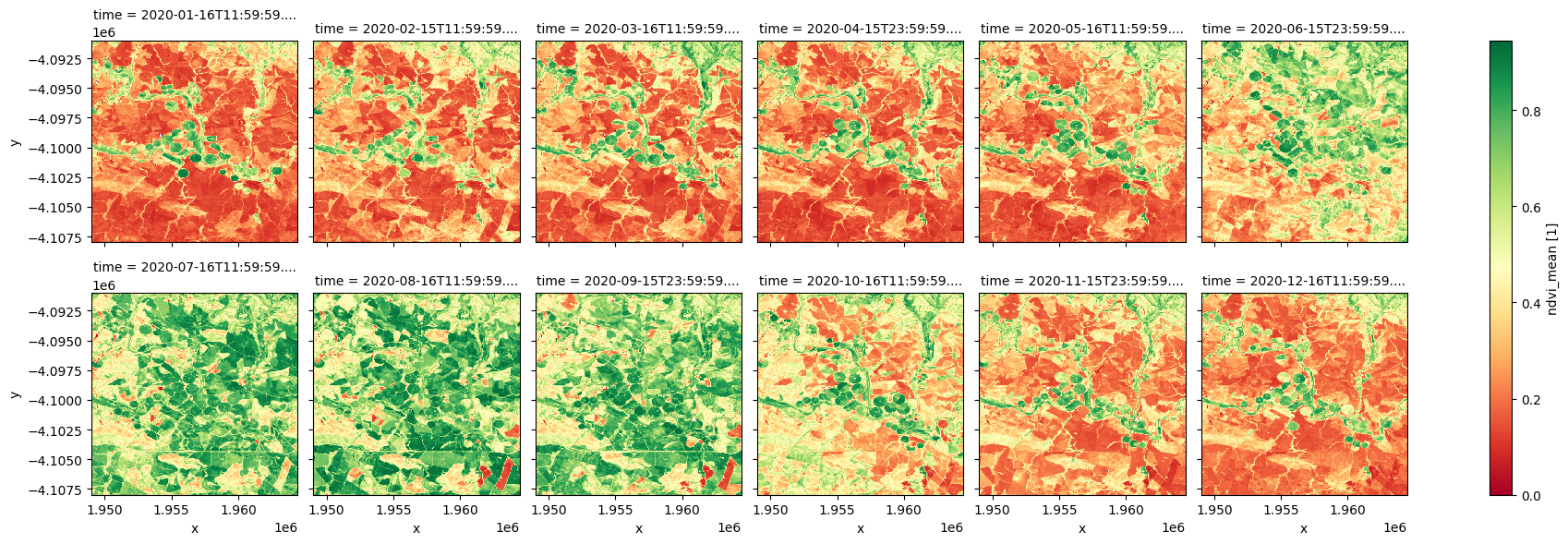
- « ndvi_mean » : NDVI moyen pour un mois.
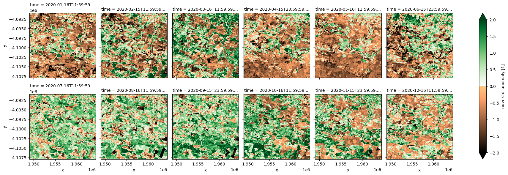
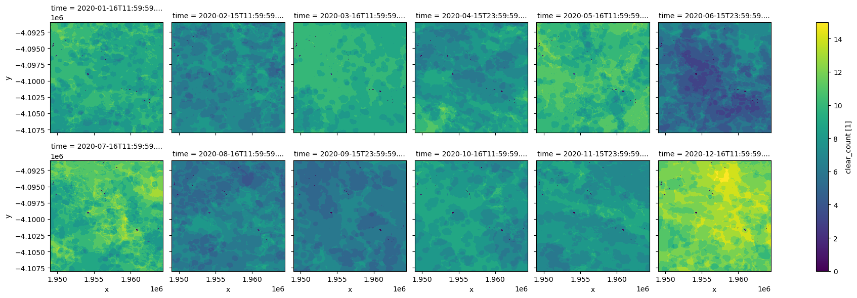
- ndvi_std_anomaly : Anomalie NDVI standardisée pour un mois
- clear_count: Nombre d’observations claires en un mois
Période : mensuelle à partir de janvier 2017
Résolution spatiale : 30 m

À partir de septembre 2022, l’anomalie mensuelle NDVI est générée sous forme de produit à faible latence, c’est-à-dire que l’anomalie d’un mois est générée le 5e jour du mois suivant. Cela garantit que les données sont disponibles peu de temps après la fin d’un mois et que toutes les observations Landsat 9 et Sentinel-2 sont incluses. Toutes les observations Landsat 8 du mois ne seront pas utilisées, car le produit Landsat 8 Surface Reflectance de l’USGS a une latence de plus de 2 semaines (voir Landsat Collection 2 Generation Timeline).

De janvier 2017 à août 2022, toutes les observations disponibles de Landsat 8, Landsat 9 et Sentinel-2 sont utilisées dans le calcul des anomalies.

Description

Dans ce bloc-notes, nous allons charger le produit NDVI et Anomalies à l’aide de dc.load() pour renvoyer la moyenne, l’écart type et le nombre d’observations claires pour chaque mois calendaire. Une dernière section explore un exemple d’analyse utilisant le produit.

Les sujets abordés comprennent :

Inspection du produit NDVI et Anomalies et des mesures disponibles dans le datacube.
Utilisation de la fonction native « dc.load() » pour charger l’anomalie NDVI pour une zone définie.
Visualisez le NDVI moyen et les anomalies standardisées.
Tracer la courbe phénologique des terres cultivées.
Extraire le NDVI moyen et les anomalies pour un mois et une région sélectionnés.
Comparez le NDVI moyen aux conditions observées au cours des années précédentes.

Commencer

Pour exécuter cette analyse, exécutez toutes les cellules du bloc-notes, en commençant par la cellule « Charger les packages ».

Charger des paquets

[1]:

import datacube
import numpy as np
import xarray as xr
import pandas as pd
import geopandas as gpd
import matplotlib as mpl
import matplotlib.pyplot as plt
import matplotlib.dates as mdates
from matplotlib.colors import ListedColormap
from odc.ui import with_ui_cbk
from odc.geo.geom import Geometry

from deafrica_tools.plotting import display_map
from deafrica_tools.spatial import xr_rasterize

Se connecter au datacube

[2]:

dc = datacube.Datacube(app='NDVI_anomaly')

Mesures disponibles

Liste des mesures

Le tableau ci-dessous présente les mesures disponibles dans le produit NDVI et Anomalies. Le NDVI moyen, l’anomalie NDVI standardisée et le nombre d’observations claires peuvent être chargés pour chaque mois calendaire.

[3]:

product_name = 'ndvi_anomaly'

dc_measurements = dc.list_measurements()
dc_measurements.loc[product_name].drop('flags_definition', axis=1)

[3]:

	name	dtype	units	nodata	aliases	scale_factor
measurement
ndvi_mean	ndvi_mean	float32	1	NaN	[NDVI_MEAN]	NaN
ndvi_std_anomaly	ndvi_std_anomaly	float32	1	NaN	[NDVI_STD_ANOMALY]	NaN
clear_count	clear_count	int8	1	0.0	[CLEAR_COUNT, count]	NaN

Paramètres d’analyse

Cette section définit les paramètres d’analyse, notamment :

« lat, lon, buffer » : latitude/longitude centrale et taille de la fenêtre d’analyse pour la zone d’intérêt.
résolution : la résolution en pixels à utiliser pour charger le ndvi_anomaly. La résolution native du produit est de 30 mètres, soit (-30,30) car le produit est dérivé de Landsat.
time_range : plage horaire pour le chargement des anomalies mensuelles.

L’emplacement par défaut est une région de culture du Cap occidental, en Afrique du Sud, où un système d’irrigation le long d’une rivière est entouré de cultures pluviales.

[4]:

lat, lon = -34.0602, 20.2800  # capetown

buffer = 0.08

resolution = (-30, 30)

# join lat, lon, buffer to get bounding box
lon_range = (lon - buffer, lon + buffer)
lat_range = (lat + buffer, lat - buffer)

time = '2020'

Afficher l’emplacement sélectionné

La cellule suivante affichera la zone sélectionnée sur une carte interactive. N’hésitez pas à zoomer et dézoomer pour mieux comprendre la zone que vous allez analyser. En cliquant sur n’importe quel point de la carte, vous découvrirez les coordonnées de latitude et de longitude de ce point.

[5]:

display_map(lon_range, lat_range)

[5]:

Make this Notebook Trusted to load map: File -> Trust Notebook

Charger les données

Ci-dessous, nous utilisons la fonction « dc.load » pour charger toutes les mesures sur la région spécifiée ci-dessus.

[6]:

# load data
ndvi_anom = dc.load(
    product="ndvi_anomaly",
    resolution=resolution,
    x=lon_range,
    y=lat_range,
    time=time,
    progress_cbk=with_ui_cbk(),
)

print(ndvi_anom)

<xarray.Dataset> Size: 32MB
Dimensions:           (time: 12, y: 567, x: 515)
Coordinates:
  * time              (time) datetime64[ns] 96B 2020-01-16T11:59:59.999999 .....
  * y                 (y) float64 5kB -4.091e+06 -4.091e+06 ... -4.108e+06
  * x                 (x) float64 4kB 1.949e+06 1.949e+06 ... 1.964e+06
    spatial_ref       int32 4B 6933
Data variables:
    ndvi_mean         (time, y, x) float32 14MB 0.4438 0.4615 ... 0.1562 0.1542
    ndvi_std_anomaly  (time, y, x) float32 14MB -0.3588 0.2575 ... -0.7113
    clear_count       (time, y, x) int8 4MB 10 11 11 11 11 11 ... 12 12 12 12 12
Attributes:
    crs:           epsg:6933
    grid_mapping:  spatial_ref

Tracé mensuel du NDVI et des anomalies

[7]:

# define  colormaps for NDVI STD Anomalies
top = mpl.colormaps['copper'].resampled(128)
bottom = mpl.colormaps['Greens'].resampled(128)
# create a new colormaps with a name of BrownGreen
newcolors = np.vstack((top(np.linspace(0, 1, 128)),
                       bottom(np.linspace(0, 1, 128))))
cramp = ListedColormap(newcolors, name='cramp')

[8]:

ndvi_anom.ndvi_mean.plot.imshow(col='time', col_wrap=6, cmap="RdYlGn");

../../../_images/sandbox_notebooks_Datasets_NDVI_Anomaly_19_0.png

[9]:

ndvi_anom.ndvi_std_anomaly.plot.imshow(col='time', col_wrap=6, cmap=cramp, vmin=-2, vmax=2);

../../../_images/sandbox_notebooks_Datasets_NDVI_Anomaly_20_0.png

[10]:

ndvi_anom.clear_count.plot.imshow(col='time', col_wrap=6, cmap="viridis");

../../../_images/sandbox_notebooks_Datasets_NDVI_Anomaly_21_0.png

Graphique phénologique NDVI

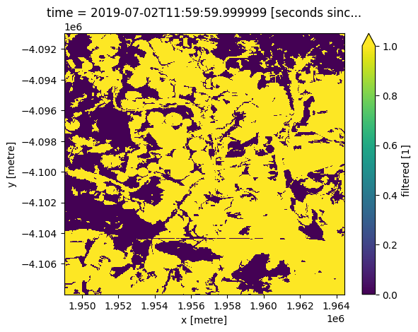
Nous pouvons utiliser le NDVI mensuel pour extraire la courbe phénologique de paysages spécifiques. En limitant notre analyse de la zone ci-dessus à un masque de culture, nous pouvons étudier la phénologie des terres cultivées.

[11]:

#Load the cropmask dataset for the region

cm = dc.load(product="crop_mask",
             measurements='filtered',
             resampling='nearest',
             like=ndvi_anom.geobox).filtered.squeeze()

cm.plot.imshow(vmin=0, vmax=1);

../../../_images/sandbox_notebooks_Datasets_NDVI_Anomaly_24_0.png

[12]:

#Mask the datasets with the crop mask
ndvi_anom_crop = ndvi_anom.where(cm)

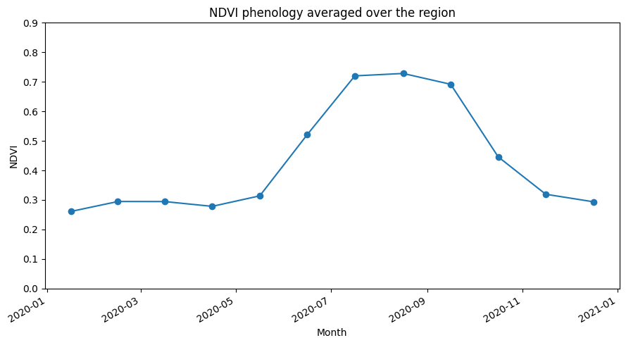
Tracer la courbe phénologique

Ci-dessous, nous résumons les ensembles de données spatialement en prenant la moyenne sur les dimensions « x » et « y ». Cela nous laissera avec la tendance moyenne au fil du temps pour la région que nous avons chargée.

À partir de la parcelle phénologique, nous pouvons conclure que la croissance des cultures dans cette zone a commencé vers mai et s’est poursuivie jusqu’à la récolte vers octobre.

Pour une analyse plus détaillée de la phénologie de la végétation, voir le carnet Vegetation Phenology notebook.

[13]:

ndvi_mean_crop = ndvi_anom_crop.ndvi_mean.mean(['x','y'])

[14]:

ndvi_mean_crop.plot(figsize=(9,5), marker='o')
plt.ylim(0,0.9)
plt.title('NDVI phenology averaged over the region')
plt.xlabel('Month')
plt.ylabel('NDVI')
plt.tight_layout()

../../../_images/sandbox_notebooks_Datasets_NDVI_Anomaly_28_0.png

Extraire les anomalies NDVI pour un mois et une région sélectionnés

[15]:

# Select a country
country = "Uganda"

# year and month for anomaly
year_month = "2022-06"

# pixel resolution can got as low as (-30,30) metres,
# but make larger for big areas.
resolution = (-120, 120)

# how to chunk the dataset for use with dask
dask_chunks = dict(x=1000, y=1000)

Charger le fichier de formes des pays africains

Ce shapefile contient des polygones pour les frontières des pays africains et nous permettra de calculer les anomalies NDVI dans un pays choisi.

[16]:

african_countries = gpd.read_file('../Supplementary_data/Rainfall_anomaly_CHIRPS/african_countries.geojson')

Liste des pays

Vous pouvez modifier le pays dans la cellule des paramètres d’analyse pour choisir n’importe quel pays africain. Une liste complète des pays est imprimée ci-dessous.

[17]:

print(np.unique(african_countries.COUNTRY))

['Algeria' 'Angola' 'Benin' 'Botswana' 'Burkina Faso' 'Burundi' 'Cameroon'
 'Cape Verde' 'Central African Republic' 'Chad' 'Comoros'
 'Congo-Brazzaville' 'Cote d`Ivoire' 'Democratic Republic of Congo'
 'Djibouti' 'Egypt' 'Equatorial Guinea' 'Eritrea' 'Ethiopia' 'Gabon'
 'Gambia' 'Ghana' 'Guinea' 'Guinea-Bissau' 'Kenya' 'Lesotho' 'Liberia'
 'Libya' 'Madagascar' 'Malawi' 'Mali' 'Mauritania' 'Morocco' 'Mozambique'
 'Namibia' 'Niger' 'Nigeria' 'Rwanda' 'Sao Tome and Principe' 'Senegal'
 'Sierra Leone' 'Somalia' 'South Africa' 'Sudan' 'Swaziland' 'Tanzania'
 'Togo' 'Tunisia' 'Uganda' 'Western Sahara' 'Zambia' 'Zimbabwe']

Configuration du polygone

Le pays sélectionné doit être transformé en objet géométrique à utiliser dans la fonction « load_ard ».

[18]:

idx = african_countries[african_countries['COUNTRY'] == country].index[0]
geom = Geometry(geom=african_countries.iloc[idx].geometry, crs=african_countries.crs)

Charger une anomalie NDVI

[19]:

ndvi_anom = dc.load(
    product="ndvi_anomaly",
    resolution=resolution,
    geopolygon=geom,
    time=year_month,
    dask_chunks=dask_chunks,
).squeeze()

print(ndvi_anom)

<xarray.Dataset> Size: 238MB
Dimensions:           (y: 6070, x: 4364)
Coordinates:
    time              datetime64[ns] 8B 2022-06-15T23:59:59.999999
  * y                 (y) float64 49kB 5.397e+05 5.396e+05 ... -1.886e+05
  * x                 (x) float64 35kB 2.853e+06 2.854e+06 ... 3.377e+06
    spatial_ref       int32 4B 6933
Data variables:
    ndvi_mean         (y, x) float32 106MB dask.array<chunksize=(1000, 1000), meta=np.ndarray>
    ndvi_std_anomaly  (y, x) float32 106MB dask.array<chunksize=(1000, 1000), meta=np.ndarray>
    clear_count       (y, x) int8 26MB dask.array<chunksize=(1000, 1000), meta=np.ndarray>
Attributes:
    crs:           epsg:6933
    grid_mapping:  spatial_ref

[20]:

african_countries = african_countries.to_crs('epsg:6933')
mask = xr_rasterize(african_countries[african_countries['COUNTRY'] == country], ndvi_anom)

[21]:

ndvi_anom = ndvi_anom.where(mask==1)

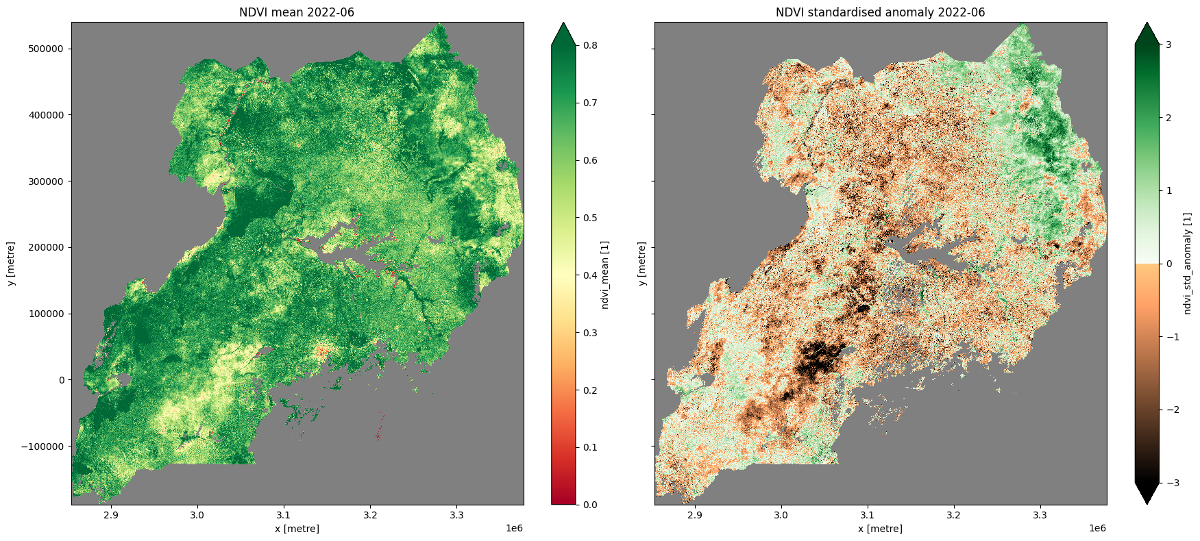
Graphique climatologique NDVI, moyenne mensuelle et anomalie standardisée

[22]:

# plot all layers
plt.rcParams["axes.facecolor"] = "gray"  # makes transparent pixels obvious
fig, ax = plt.subplots(1, 2, sharey=True, sharex=True, figsize=(18, 8))

ndvi_anom.ndvi_mean.plot.imshow(ax=ax[0], cmap="RdYlGn",vmin=0,vmax=0.8)
ax[0].set_title("NDVI mean " + year_month)

ndvi_anom.ndvi_std_anomaly.plot.imshow(ax=ax[1], cmap=cramp, vmin=-3, vmax=3)
ax[1].set_title("NDVI standardised anomaly " + year_month)
plt.tight_layout();

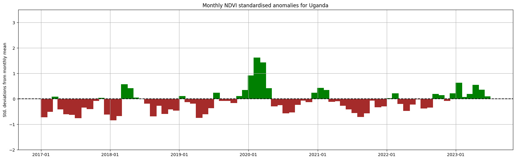
../../../_images/sandbox_notebooks_Datasets_NDVI_Anomaly_42_0.png

Comparer les conditions mensuelles du NDVI au fil des ans

[23]:

ndvi_anom = dc.load(
    product="ndvi_anomaly",
    resolution=resolution,
    geopolygon=geom,
#     time=year_month,
    dask_chunks=dask_chunks,
)

Ci-dessous, la moyenne spatiale est prise afin que nous puissions présenter les anomalies mensuelles agrégées sur l’ensemble du pays sélectionné.

[24]:

spatial_mean_anoms = ndvi_anom.ndvi_std_anomaly.mean(['x','y']).to_dataframe().drop(['spatial_ref'], axis=1)

[25]:

plt.rcParams["axes.facecolor"] = "white"
fig, ax = plt.subplots(figsize=(21,6))
ax.xaxis.set_major_formatter(mdates.DateFormatter("%Y-%m"))
ax.set_ylim(-2,3.5)
ax.bar(spatial_mean_anoms.index,
       spatial_mean_anoms.ndvi_std_anomaly,
       width=35, align='center',
       color=(spatial_mean_anoms['ndvi_std_anomaly'] > 0).map({True: 'g', False: 'brown'}))
ax.axhline(0, color='black', linestyle='--')
plt.title('Monthly NDVI standardised anomalies for '+ country)
plt.ylabel('Std. deviations from monthly mean');
plt.grid()

../../../_images/sandbox_notebooks_Datasets_NDVI_Anomaly_48_0.png

Informations Complémentaires

Licence : Le code de ce carnet est sous licence Apache, version 2.0 <https://www.apache.org/licenses/LICENSE-2.0>. Les données de Digital Earth Africa sont sous licence Creative Commons par attribution 4.0 <https://creativecommons.org/licenses/by/4.0/>.

Contact : Si vous avez besoin d’aide, veuillez poster une question sur le canal Slack Open Data Cube <http://slack.opendatacube.org/>`__ ou sur le GIS Stack Exchange en utilisant la balise open-data-cube (vous pouvez consulter les questions posées précédemment ici). Si vous souhaitez signaler un problème avec ce bloc-notes, vous pouvez en déposer un sur Github.

Version de Datacube compatible :

[26]:

print(datacube.__version__)

1.8.20

Dernier test :

[27]:

from datetime import datetime
datetime.today().strftime('%Y-%m-%d')

[27]:

'2025-01-15'