Données sur les sols de l’iSDA

• Produits utilisés : iSDA Soil

Mots clés données utilisées ; iSDA soil, soil, données utilisées ; isda_soil_bedrock_depth, données utilisées ; isda_soil_bulk_density, données utilisées ; isda_soil_carbon_total, données utilisées ; isda_soil_clay_content, données utilisées ; isda_soil_sand_content, données utilisées ; isda_soil_silt_content,

Aperçu

iSDAsoil <https://www.isda-africa.com/isdasoil/>`__ est une ressource de données sur les sols en libre accès pour le continent africain. Les données sur les sols peuvent être utiles pour une gamme d’applications, notamment la cartographie de l’aptitude des terres à l’agriculture, la planification de l’amélioration des sols (par exemple, le chaulage pour traiter les sols acides ou l’engrais pour répondre aux contraintes de fertilité) et la planification de la construction/des infrastructures.

Description

Ce bloc-notes montre comment intégrer ces données aux produits et flux de travail de DE Africa. Pour des informations techniques sur iSDAsoil, voir Miller et al. 2021. Une partie du code de ce bloc-notes a été adaptée à partir du GitHub iSDA-Africa.

1. Charger les données iSDA

2. Visualisez l’iSDA par rapport aux produits DE Africa

---

Commencer

Pour exécuter cette analyse, exécutez toutes les cellules du bloc-notes, en commençant par la cellule « Charger les packages ».

Charger des paquets

Importez les packages Python utilisés pour l’analyse.

Notez que nous chargeons un module appelé « load_isda() » pour ce notebook qui prend un peu de temps à charger.

%matplotlib inline

import datacube
import numpy as np
import pandas as pd
import xarray as xr
import matplotlib.pyplot as plt
import matplotlib.patches as mpatches
import rasterio as rio
from pyproj import Transformer
import matplotlib.pyplot as plt
import os
import numpy as np

from urllib.parse import urlparse
import boto3
from pystac import stac_io, Catalog
from deafrica_tools.plotting import display_map, rgb
from deafrica_tools.load_isda import load_isda

Se connecter au datacube

dc = datacube.Datacube(app='iSDA-soil')

Variables iSDA

iSDA propose de nombreuses variables de sol présentées dans le tableau ci-dessous. La plupart des variables ont quatre couches : moyenne et écart type à 0-20 cm et 20-5 cm de profondeur. Nous verrons à travers le bloc-notes que nous pouvons introduire chaque variable avec les noms d’accès, par exemple « bedrock_depth ».

Certaines variables sont indexées dans Digital Earth Africa, et d’autres peuvent être importées directement.

Variable	Nom d’accès	Couches
Aluminium extractible	aluminium_extractible	0-20 cm et 20-50 cm, moyenne prédite et écart type
Profondeur du substrat rocheux	profondeur_du_substrat_rocheux	Profondeur de 0 à 200 cm, moyenne prévue et écart type
Densité apparente, fraction < 2 mm	densité volumique	0-20 cm et 20-50 cm, moyenne prédite et écart type
Calcium extractible	calcium_extractible	0-20 cm et 20-50 cm, moyenne prédite et écart type
Carbone organique	carbone_organique	0-20 cm et 20-50 cm, moyenne prédite et écart type
Carbone total	carbone_total	0-20 cm et 20-50 cm, moyenne prédite et écart type
Capacité d’échange de cations efficace	capacité d’échange de cations	0-20 cm et 20-50 cm, moyenne prédite et écart type
Teneur en argile	argile_contenu	0-20 cm et 20-50 cm, moyenne prédite et écart type
Classification de la capacité de fertilité	FCC	Couche de classification unique
Fer extractible	extractible_de_fer	0-20 cm et 20-50 cm, moyenne prédite et écart type
Magnésium, extractible	magnésium_extractible	0-20 cm et 20-50 cm, moyenne prédite et écart type
Azote total	azote_total	0-20 cm et 20-50 cm, moyenne prédite et écart type
pH	ph	0-20 cm et 20-50 cm, moyenne prédite et écart type
Phosphore, extractible	phosphore_extractible	0-20 cm et 20-50 cm, moyenne prédite et écart type
Potassium extractible	extractible au potassium	0-20 cm et 20-50 cm, moyenne prédite et écart type
Teneur en sable	contenu_sable	0-20 cm et 20-50 cm, moyenne prédite et écart type
Teneur en limon	teneur en limon	0-20 cm et 20-50 cm, moyenne prédite et écart type
Teneur en pierre	contenu_en_pierre	Des fragments grossiers sont prévus à une profondeur de 0 à 20 cm
Soufre extractible	extractible au soufre	0-20 cm et 20-50 cm, moyenne prédite et écart type
Classe de texture USDA	classe_de_texture	0-20 cm et 20-50 cm de profondeur, moyenne prévue
Zinc, extractible	zinc_extractible	0-20 cm et 20-50 cm, moyenne prédite et écart type

Données sur les sols indexées

Il existe six ensembles de données de sol iSDA indexés par Digital Earth Africa et disponibles pour un chargement direct.

# List iSDA products available in DE Africa
dc_products = dc.list_products()
display_columns = ['name', 'description']
dc_products[dc_products.name.str.contains(
    'soil').fillna(
        False)][display_columns].set_index('name')

	description
name
isda_soil_bedrock_depth	Soil bedrock depth predictions made by iSDA Af...
isda_soil_bulk_density	Soil bulk density predictions made by iSDA Africa
isda_soil_carbon_total	Soil total carbon predictions made by iSDA Africa
isda_soil_clay_content	Soil clay content predictions made by iSDA Africa
isda_soil_sand_content	Soil sand content predictions made by iSDA Africa
isda_soil_silt_content	Soil silt content predictions made by iSDA Africa

Liste des mesures

De nombreux produits sur les sols comportent des mesures pour deux profondeurs : 0-20 cm et 20-50 cm. Ils comportent également des estimations moyennes et des écarts types, comme indiqué ci-dessous pour le carbone total du sol.

product_name = 'isda_soil_carbon_total'

dc_measurements = dc.list_measurements()
dc_measurements.loc[product_name].drop('flags_definition', axis=1)

	name	dtype	units	nodata	aliases
measurement
mean_0_20	mean_0_20	float32	g/kg	NaN	[MEAN_0_20]
mean_20_50	mean_20_50	float32	g/kg	NaN	[MEAN_20_50]
stdev_0_20	stdev_0_20	float32	g/kg	NaN	[STDEV_0_20]
stdev_20_50	stdev_20_50	float32	g/kg	NaN	[STDEV_20_50]

Définir les paramètres

Définissons quelques paramètres pour le chargement des données sur le carbone du sol pour une zone côtière près du Cap, en Afrique du Sud.

lat = -32.9
lon = 18.7
buffer = 0.5

display_map((lon - buffer, lon + buffer), (lat - buffer, lat + buffer))

Make this Notebook Trusted to load map: File -> Trust Notebook

Charger les données de sol iSDA à l’aide de dc.load()

Maintenant que nous savons quels produits et mesures sont disponibles, nous pouvons charger des données à partir du datacube en utilisant « dc.load ».

# load data
ds = dc.load(product="isda_soil_carbon_total",
             measurements=['mean_0_20', 'mean_20_50', 'stdev_0_20', 'stdev_20_50'],
             x=(lon - buffer, lon + buffer),
             y=(lat - buffer, lat + buffer)
             )

ds

<xarray.Dataset>
Dimensions:      (time: 1, y: 4421, x: 3712)
Coordinates:
  * time         (time) datetime64[ns] 2009-01-01
  * y            (y) float64 -3.816e+06 -3.816e+06 ... -3.948e+06 -3.949e+06
  * x            (x) float64 2.026e+06 2.026e+06 ... 2.137e+06 2.137e+06
    spatial_ref  int32 3857
Data variables:
    mean_0_20    (time, y, x) float32 nan nan nan nan ... 28.0 29.0 28.0 28.0
    mean_20_50   (time, y, x) float32 nan nan nan nan ... 26.0 26.0 27.0 25.0
    stdev_0_20   (time, y, x) float32 nan nan nan nan nan ... 5.0 5.0 5.0 5.0
    stdev_20_50  (time, y, x) float32 nan nan nan nan nan ... 3.0 3.0 3.0 3.0
Attributes:
    crs:           EPSG:3857
    grid_mapping:  spatial_ref

xarray.Dataset

• Dimensions:
  • time: 1
  • y: 4421
  • x: 3712
• Coordinates: (4)
  • time
    (time)
    datetime64[ns]
    2009-01-01

    units :

    seconds since 1970-01-01 00:00:00

    array(['2009-01-01T00:00:00.000000000'], dtype='datetime64[ns]')

  • y
    (y)
    float64
    -3.816e+06 ... -3.949e+06

    units :

    metre

    resolution :

    -30.0

    crs :

    EPSG:3857

    array([-3815925., -3815955., -3815985., ..., -3948465., -3948495., -3948525.])

  • x
    (x)
    float64
    2.026e+06 2.026e+06 ... 2.137e+06

    units :

    metre

    resolution :

    30.0

    crs :

    EPSG:3857

    array([2026005., 2026035., 2026065., ..., 2137275., 2137305., 2137335.])

  • spatial_ref
    ()
    int32
    3857

    spatial_ref :

    PROJCS["WGS 84 / Pseudo-Mercator",GEOGCS["WGS 84",DATUM["WGS_1984",SPHEROID["WGS 84",6378137,298.257223563,AUTHORITY["EPSG","7030"]],AUTHORITY["EPSG","6326"]],PRIMEM["Greenwich",0,AUTHORITY["EPSG","8901"]],UNIT["degree",0.0174532925199433,AUTHORITY["EPSG","9122"]],AUTHORITY["EPSG","4326"]],PROJECTION["Mercator_1SP"],PARAMETER["central_meridian",0],PARAMETER["scale_factor",1],PARAMETER["false_easting",0],PARAMETER["false_northing",0],UNIT["metre",1,AUTHORITY["EPSG","9001"]],AXIS["Easting",EAST],AXIS["Northing",NORTH],EXTENSION["PROJ4","+proj=merc +a=6378137 +b=6378137 +lat_ts=0 +lon_0=0 +x_0=0 +y_0=0 +k=1 +units=m +nadgrids=@null +wktext +no_defs"],AUTHORITY["EPSG","3857"]]

    grid_mapping_name :

    ??

    array(3857, dtype=int32)

• Data variables: (4)
  • mean_0_20
    (time, y, x)
    float32
    nan nan nan nan ... 29.0 28.0 28.0

    units :

    g/kg

    nodata :

    nan

    flags_definition :

    {'back-transformation': 'expm1(x/10)'}

    crs :

    EPSG:3857

    grid_mapping :

    spatial_ref

    array([[[nan, nan, nan, ..., 28., 28., 28.],
            [nan, nan, nan, ..., 27., 27., 28.],
            [nan, nan, nan, ..., 27., 27., 28.],
            ...,
            [nan, nan, nan, ..., 29., 28., 28.],
            [nan, nan, nan, ..., 29., 28., 28.],
            [nan, nan, nan, ..., 29., 28., 28.]]], dtype=float32)

  • mean_20_50
    (time, y, x)
    float32
    nan nan nan nan ... 26.0 27.0 25.0

    units :

    g/kg

    nodata :

    nan

    flags_definition :

    {'back-transformation': 'expm1(x/10)'}

    crs :

    EPSG:3857

    grid_mapping :

    spatial_ref

    array([[[nan, nan, nan, ..., 27., 27., 27.],
            [nan, nan, nan, ..., 26., 26., 27.],
            [nan, nan, nan, ..., 26., 26., 27.],
            ...,
            [nan, nan, nan, ..., 27., 26., 26.],
            [nan, nan, nan, ..., 27., 26., 26.],
            [nan, nan, nan, ..., 26., 27., 25.]]], dtype=float32)

  • stdev_0_20
    (time, y, x)
    float32
    nan nan nan nan ... 5.0 5.0 5.0 5.0

    units :

    g/kg

    nodata :

    nan

    flags_definition :

    {'back-transformation': 'expm1(x/10)'}

    crs :

    EPSG:3857

    grid_mapping :

    spatial_ref

    array([[[nan, nan, nan, ...,  2.,  2.,  1.],
            [nan, nan, nan, ...,  2.,  2.,  2.],
            [nan, nan, nan, ...,  2.,  2.,  2.],
            ...,
            [nan, nan, nan, ...,  5.,  5.,  5.],
            [nan, nan, nan, ...,  5.,  5.,  5.],
            [nan, nan, nan, ...,  5.,  5.,  5.]]], dtype=float32)

  • stdev_20_50
    (time, y, x)
    float32
    nan nan nan nan ... 3.0 3.0 3.0 3.0

    units :

    g/kg

    nodata :

    nan

    flags_definition :

    {'back-transformation': 'expm1(x/10)'}

    crs :

    EPSG:3857

    grid_mapping :

    spatial_ref

    array([[[nan, nan, nan, ...,  1.,  1.,  1.],
            [nan, nan, nan, ...,  2.,  2.,  1.],
            [nan, nan, nan, ...,  2.,  2.,  1.],
            ...,
            [nan, nan, nan, ...,  3.,  4.,  4.],
            [nan, nan, nan, ...,  3.,  3.,  3.],
            [nan, nan, nan, ...,  3.,  3.,  3.]]], dtype=float32)

• Indexes: (3)
  • time
    PandasIndex

    PandasIndex(DatetimeIndex(['2009-01-01'], dtype='datetime64[ns]', name='time', freq=None))

  • y
    PandasIndex

    PandasIndex(Index([-3815925.0, -3815955.0, -3815985.0, -3816015.0, -3816045.0, -3816075.0,
           -3816105.0, -3816135.0, -3816165.0, -3816195.0,
           ...
           -3948255.0, -3948285.0, -3948315.0, -3948345.0, -3948375.0, -3948405.0,
           -3948435.0, -3948465.0, -3948495.0, -3948525.0],
          dtype='float64', name='y', length=4421))

  • x
    PandasIndex

    PandasIndex(Index([2026005.0, 2026035.0, 2026065.0, 2026095.0, 2026125.0, 2026155.0,
           2026185.0, 2026215.0, 2026245.0, 2026275.0,
           ...
           2137065.0, 2137095.0, 2137125.0, 2137155.0, 2137185.0, 2137215.0,
           2137245.0, 2137275.0, 2137305.0, 2137335.0],
          dtype='float64', name='x', length=3712))

• Attributes: (2)

  crs :

  EPSG:3857

  grid_mapping :

  spatial_ref

Appliquer la transformation

Il est important de noter qu’une grande partie des données iSDA doivent être transformées avant d’être appliquées. Pour les ensembles de données indexés, nous pouvons obtenir des métadonnées de conversion associées à chaque variable dans « flags_definition ». Cette opération est effectuée pour notre variable sélectionnée ci-dessous.

ds.mean_0_20.flags_definition

{'back-transformation': 'expm1(x/10)'}

ds = np.expm1(ds/10)

Informations sur le sol de la parcelle

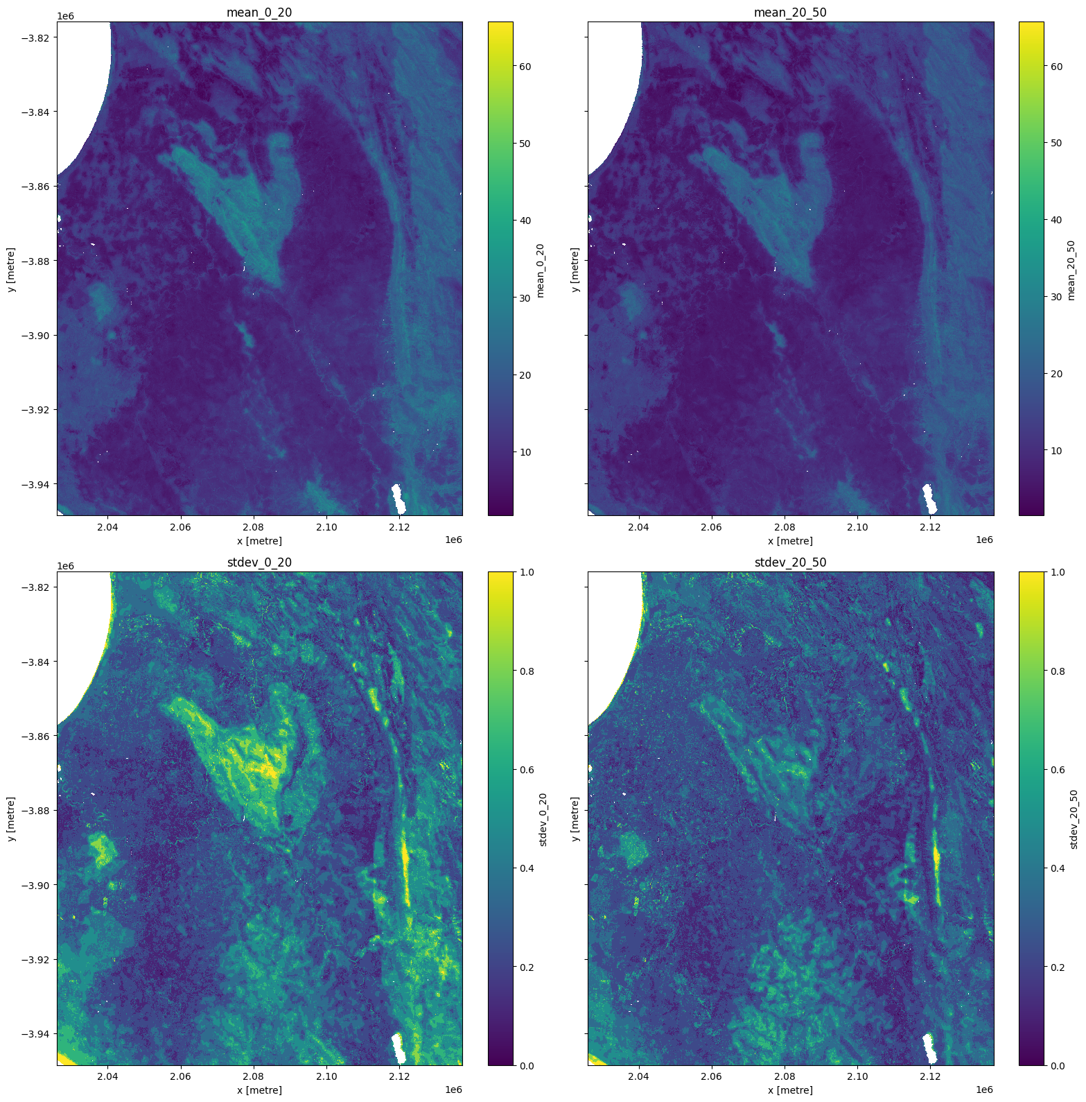
Les graphiques ci-dessous montrent le carbone du sol en g/kg. Certaines valeurs aberrantes sont évidentes dans les produits d’écart type, nous utilisons donc « clip(0,1) » pour tracer une plage raisonnable.

fig, ax = plt.subplots(2, 2, figsize=(16, 16), sharey=True)
ds[list(ds.keys())[0]].plot(ax=ax[0, 0])
ds[list(ds.keys())[1]].plot(ax=ax[0, 1])
ds[list(ds.keys())[2]].clip(0,1).plot(ax=ax[1, 0])
ds[list(ds.keys())[3]].clip(0,1).plot(ax=ax[1, 1])
ax[0, 0].set_title(list(ds.keys())[0])
ax[0, 1].set_title(list(ds.keys())[1])
ax[1, 0].set_title(list(ds.keys())[2])
ax[1, 1].set_title(list(ds.keys())[3])
plt.tight_layout();

Charger les données iSDA à partir de la source

Comme nous l’avons vu dans les sections d’introduction de ce carnet, il existe six variables iSDA indexées par Digital Earth Africa pour le chargement à l’aide de « dc.load ».

D’autres ensembles de données iSDA peuvent être chargés à partir de la source. Cette méthode de chargement présente toutefois certaines complexités, car il faut accéder aux métadonnées pour identifier les transformations et il faut également attribuer une projection spatiale.

Lien vers les métadonnées iSDA

Il existe quelques complexités associées aux données iSDA, telles que les rétrotransformations/conversions que nous verrons plus tard dans le bloc-notes. Nous devons établir un lien avec les métadonnées pour pouvoir les explorer.

La cellule ci-dessous fournit un lien vers les métadonnées nécessaires.

#this function allows us to directly query the data on s3
def my_read_method(uri):
    parsed = urlparse(uri)
    if parsed.scheme == 's3':
        bucket = parsed.netloc
        key = parsed.path[1:]
        s3 = boto3.resource('s3')
        obj = s3.Object(bucket, key)
        return obj.get()['Body'].read().decode('utf-8')
    else:
        return stac_io.default_read_text_method(uri)

stac_io.read_text_method = my_read_method

catalog = Catalog.from_file("https://isdasoil.s3.amazonaws.com/catalog.json")

assets = {}

for root, catalogs, items in catalog.walk():
    for item in items:
        str(f"Type: {item.get_parent().title}")
        # save all items to a dictionary as we go along
        assets[item.id] = item
        for asset in item.assets.values():
            if asset.roles == ['data']:
                str(f"Title: {asset.title}")
                str(f"Description: {asset.description}")
                str(f"URL: {asset.href}")
                str("------------")

Classification de la capacité de fertilité de charge

La cellule ci-dessous utilise la fonction « load_isda() » pour importer la classification des capacités de fertilité pour la zone définie ci-dessus.

Nous pouvons voir ci-dessous que la fonction renvoie une variable appelée « band_data » sous la forme « float32 ».

var = "fcc"

ds = load_isda(var, (lat-buffer, lat + buffer), (lon-buffer, lon + buffer))
ds

<xarray.Dataset>
Dimensions:      (x: 3712, y: 4420)
Coordinates:
    band         int64 1
  * x            (x) float64 2.026e+06 2.026e+06 ... 2.137e+06 2.137e+06
  * y            (y) float64 -3.816e+06 -3.816e+06 ... -3.948e+06 -3.949e+06
    spatial_ref  int64 0
Data variables:
    band_data    (y, x) float32 ...

xarray.Dataset

• Dimensions:
  • x: 3712
  • y: 4420
• Coordinates: (4)
  • band
    ()
    int64
    1

    array(1)

  • x
    (x)
    float64
    2.026e+06 2.026e+06 ... 2.137e+06

    axis :

    X

    long_name :

    x coordinate of projection

    standard_name :

    projection_x_coordinate

    units :

    metre

    array([2026012.192357, 2026042.192357, 2026072.192357, ..., 2137282.192357,
           2137312.192357, 2137342.192357])

  • y
    (y)
    float64
    -3.816e+06 ... -3.949e+06

    axis :

    Y

    long_name :

    y coordinate of projection

    standard_name :

    projection_y_coordinate

    units :

    metre

    array([-3815941.869548, -3815971.869548, -3816001.869548, ..., -3948451.869548,
           -3948481.869548, -3948511.869548])

  • spatial_ref
    ()
    int64
    0

    crs_wkt :

    PROJCS["WGS 84 / Pseudo-Mercator",GEOGCS["WGS 84",DATUM["WGS_1984",SPHEROID["WGS 84",6378137,298.257223563,AUTHORITY["EPSG","7030"]],AUTHORITY["EPSG","6326"]],PRIMEM["Greenwich",0,AUTHORITY["EPSG","8901"]],UNIT["degree",0.0174532925199433,AUTHORITY["EPSG","9122"]],AUTHORITY["EPSG","4326"]],PROJECTION["Mercator_1SP"],PARAMETER["central_meridian",0],PARAMETER["scale_factor",1],PARAMETER["false_easting",0],PARAMETER["false_northing",0],UNIT["metre",1,AUTHORITY["EPSG","9001"]],AXIS["Easting",EAST],AXIS["Northing",NORTH],EXTENSION["PROJ4","+proj=merc +a=6378137 +b=6378137 +lat_ts=0 +lon_0=0 +x_0=0 +y_0=0 +k=1 +units=m +nadgrids=@null +wktext +no_defs"],AUTHORITY["EPSG","3857"]]

    spatial_ref :

    PROJCS["WGS 84 / Pseudo-Mercator",GEOGCS["WGS 84",DATUM["WGS_1984",SPHEROID["WGS 84",6378137,298.257223563,AUTHORITY["EPSG","7030"]],AUTHORITY["EPSG","6326"]],PRIMEM["Greenwich",0,AUTHORITY["EPSG","8901"]],UNIT["degree",0.0174532925199433,AUTHORITY["EPSG","9122"]],AUTHORITY["EPSG","4326"]],PROJECTION["Mercator_1SP"],PARAMETER["central_meridian",0],PARAMETER["scale_factor",1],PARAMETER["false_easting",0],PARAMETER["false_northing",0],UNIT["metre",1,AUTHORITY["EPSG","9001"]],AXIS["Easting",EAST],AXIS["Northing",NORTH],EXTENSION["PROJ4","+proj=merc +a=6378137 +b=6378137 +lat_ts=0 +lon_0=0 +x_0=0 +y_0=0 +k=1 +units=m +nadgrids=@null +wktext +no_defs"],AUTHORITY["EPSG","3857"]]

    GeoTransform :

    2025997.1923569688 30.0 0.0 -3815926.86954757 0.0 -30.0

    array(0)

• Data variables: (1)
  • band_data
    (y, x)
    float32
    ...

    AREA_OR_POINT :

    Area

    [16407040 values with dtype=float32]

• Indexes: (2)
  • x
    PandasIndex

    PandasIndex(Index([2026012.1923569688, 2026042.1923569688, 2026072.1923569688,
           2026102.1923569688, 2026132.1923569688, 2026162.1923569688,
           2026192.1923569688, 2026222.1923569688, 2026252.1923569688,
           2026282.1923569688,
           ...
           2137072.1923569688, 2137102.1923569688, 2137132.1923569688,
           2137162.1923569688, 2137192.1923569688, 2137222.1923569688,
           2137252.1923569688, 2137282.1923569688, 2137312.1923569688,
           2137342.1923569688],
          dtype='float64', name='x', length=3712))

  • y
    PandasIndex

    PandasIndex(Index([-3815941.86954757, -3815971.86954757, -3816001.86954757,
           -3816031.86954757, -3816061.86954757, -3816091.86954757,
           -3816121.86954757, -3816151.86954757, -3816181.86954757,
           -3816211.86954757,
           ...
           -3948241.86954757, -3948271.86954757, -3948301.86954757,
           -3948331.86954757, -3948361.86954757, -3948391.86954757,
           -3948421.86954757, -3948451.86954757, -3948481.86954757,
           -3948511.86954757],
          dtype='float64', name='y', length=4420))

• Attributes: (0)

Appliquer la transformation

Il est important de noter qu’une grande partie des données iSDA doivent être transformées avant d’être appliquées. Nous pouvons utiliser l’objet que nous avons stocké appelé « assets » pour obtenir les métadonnées de conversion associées à chaque variable. Cette opération est effectuée pour notre variable sélectionnée ci-dessous.

Nous pouvons voir que la variable « fcc » renvoie une valeur de conversion de « %3000 ».

conversion = assets[var].extra_fields["back-transformation"]
conversion

'%3000'

Ci-dessous, la transformation est effectuée et une nouvelle bande est ajoutée à l’ensemble de données. Les valeurs sont converties en nombres entiers pour une interprétation et un traçage plus faciles.

ds = ds.assign(fcc = (ds["band_data"]%3000).fillna(2535).astype('int16'))

Les étiquettes peuvent également être tirées des métadonnées. Ci-dessous, les classes de fertilité sont mappées à leurs entiers respectifs pour un meilleur traçage des résultats.

fcc_labels = pd.read_csv(assets['fcc'].assets["metadata"].href, index_col=0)

mappings = {val:fcc_labels.loc[int(val),"Description"] for val in np.unique(ds.fcc.astype('int16'))}

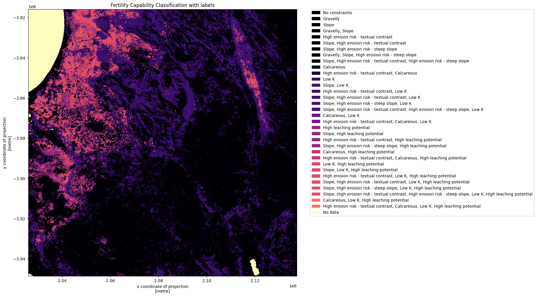
Classification de la capacité de fertilité des parcelles

Nous pouvons maintenant tracer les données « fcc » avec des étiquettes.

plt.figure(figsize=(12,12), dpi= 100)
im = ds.fcc.plot(cmap="magma", add_colorbar=False)
colors = [ im.cmap(im.norm(value)) for value in np.unique(ds.fcc)]
patches = [mpatches.Patch(color=colors[idx], label=str(mappings[val])) for idx, val in enumerate(np.unique(ds.fcc))]
plt.legend(handles=patches, bbox_to_anchor=(1.05, 1), loc=2, borderaxespad=0. )
plt.title("Fertility Capability Classification with labels")
plt.show()

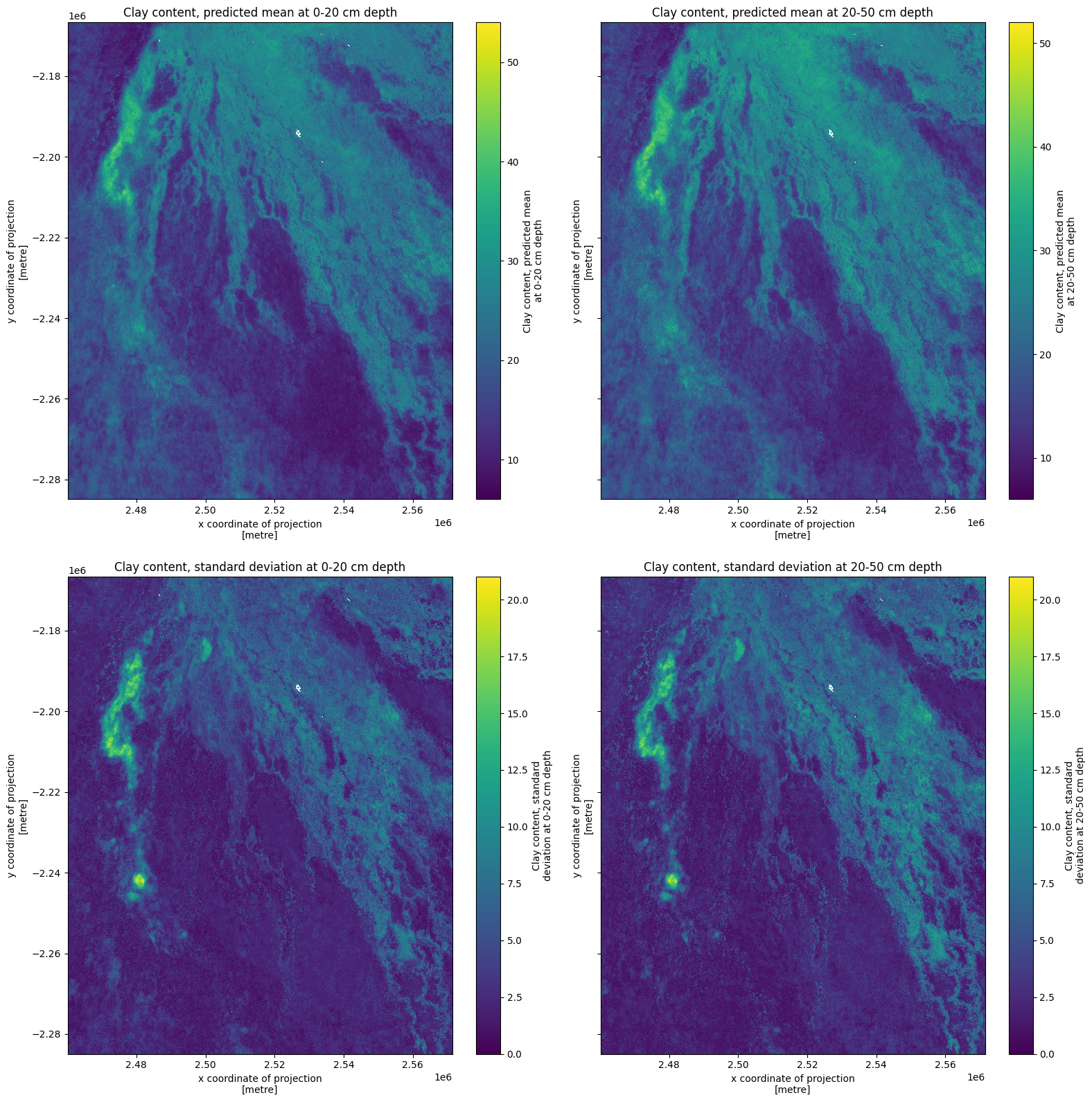
Argile dans le delta de l’Okavango

Nous allons maintenant inspecter la teneur en argile du sol dans le delta de l’Okavango, au Botswana.

Nouveaux paramètres

De nouveaux paramètres pour le chargement des données sont définis dans la cellule ci-dessous. L’objet « var » est extrait du nom d’accès correspondant indiqué au début de ce bloc-notes.

var = 'clay_content'

lat = -19.6
lon = 22.6
buffer = 0.5

display_map((lon - buffer, lon + buffer), (lat - buffer, lat + buffer))

Make this Notebook Trusted to load map: File -> Trust Notebook

Utilisez la fonction « load_isda() » pour importer les données sur le contenu en argile.

ds = load_isda(var, (lat-buffer, lat + buffer), (lon-buffer, lon + buffer))
ds

/usr/local/lib/python3.10/dist-packages/rioxarray/_io.py:430: NodataShadowWarning: The dataset's nodata attribute is shadowing the alpha band. All masks will be determined by the nodata attribute
  out = riods.read(band_key, window=window, masked=self.masked)
/usr/local/lib/python3.10/dist-packages/rioxarray/_io.py:430: NodataShadowWarning: The dataset's nodata attribute is shadowing the alpha band. All masks will be determined by the nodata attribute
  out = riods.read(band_key, window=window, masked=self.masked)
/usr/local/lib/python3.10/dist-packages/rioxarray/_io.py:430: NodataShadowWarning: The dataset's nodata attribute is shadowing the alpha band. All masks will be determined by the nodata attribute
  out = riods.read(band_key, window=window, masked=self.masked)
/usr/local/lib/python3.10/dist-packages/rioxarray/_io.py:430: NodataShadowWarning: The dataset's nodata attribute is shadowing the alpha band. All masks will be determined by the nodata attribute
  out = riods.read(band_key, window=window, masked=self.masked)

<xarray.Dataset>
Dimensions:                                             (x: 3711, y: 3940)
Coordinates:
  * x                                                   (x) float64 2.46e+06 ...
  * y                                                   (y) float64 -2.167e+0...
    spatial_ref                                         int64 0
    band                                                <U9 'band_data'
Data variables:
    Clay content, predicted mean at 0-20 cm depth       (y, x) float32 13.0 ....
    Clay content, predicted mean at 20-50 cm depth      (y, x) float32 13.0 ....
    Clay content, standard deviation at 0-20 cm depth   (y, x) float32 2.0 .....
    Clay content, standard deviation at 20-50 cm depth  (y, x) float32 2.0 .....

xarray.Dataset

• Dimensions:
  • x: 3711
  • y: 3940
• Coordinates: (4)
  • x
    (x)
    float64
    2.46e+06 2.46e+06 ... 2.571e+06

    axis :

    X

    long_name :

    x coordinate of projection

    standard_name :

    projection_x_coordinate

    units :

    metre

    array([2460172.192357, 2460202.192357, 2460232.192357, ..., 2571412.192357,
           2571442.192357, 2571472.192357])

  • y
    (y)
    float64
    -2.167e+06 ... -2.285e+06

    axis :

    Y

    long_name :

    y coordinate of projection

    standard_name :

    projection_y_coordinate

    units :

    metre

    array([-2166721.869548, -2166751.869548, -2166781.869548, ..., -2284831.869548,
           -2284861.869548, -2284891.869548])

  • spatial_ref
    ()
    int64
    0

    crs_wkt :

    PROJCS["WGS 84 / Pseudo-Mercator",GEOGCS["WGS 84",DATUM["WGS_1984",SPHEROID["WGS 84",6378137,298.257223563,AUTHORITY["EPSG","7030"]],AUTHORITY["EPSG","6326"]],PRIMEM["Greenwich",0,AUTHORITY["EPSG","8901"]],UNIT["degree",0.0174532925199433,AUTHORITY["EPSG","9122"]],AUTHORITY["EPSG","4326"]],PROJECTION["Mercator_1SP"],PARAMETER["central_meridian",0],PARAMETER["scale_factor",1],PARAMETER["false_easting",0],PARAMETER["false_northing",0],UNIT["metre",1,AUTHORITY["EPSG","9001"]],AXIS["Easting",EAST],AXIS["Northing",NORTH],EXTENSION["PROJ4","+proj=merc +a=6378137 +b=6378137 +lat_ts=0 +lon_0=0 +x_0=0 +y_0=0 +k=1 +units=m +nadgrids=@null +wktext +no_defs"],AUTHORITY["EPSG","3857"]]

    spatial_ref :

    PROJCS["WGS 84 / Pseudo-Mercator",GEOGCS["WGS 84",DATUM["WGS_1984",SPHEROID["WGS 84",6378137,298.257223563,AUTHORITY["EPSG","7030"]],AUTHORITY["EPSG","6326"]],PRIMEM["Greenwich",0,AUTHORITY["EPSG","8901"]],UNIT["degree",0.0174532925199433,AUTHORITY["EPSG","9122"]],AUTHORITY["EPSG","4326"]],PROJECTION["Mercator_1SP"],PARAMETER["central_meridian",0],PARAMETER["scale_factor",1],PARAMETER["false_easting",0],PARAMETER["false_northing",0],UNIT["metre",1,AUTHORITY["EPSG","9001"]],AXIS["Easting",EAST],AXIS["Northing",NORTH],EXTENSION["PROJ4","+proj=merc +a=6378137 +b=6378137 +lat_ts=0 +lon_0=0 +x_0=0 +y_0=0 +k=1 +units=m +nadgrids=@null +wktext +no_defs"],AUTHORITY["EPSG","3857"]]

    GeoTransform :

    2460157.1923569688 30.0 0.0 -2166706.86954757 0.0 -30.0

    array(0)

  • band
    ()
    <U9
    'band_data'

    array('band_data', dtype='<U9')

• Data variables: (4)
  • Clay content, predicted mean at 0-20 cm depth
    (y, x)
    float32
    13.0 14.0 15.0 ... 11.0 12.0 12.0

    array([[13., 14., 15., ..., 26., 26., 26.],
           [14., 15., 15., ..., 28., 26., 26.],
           [17., 14., 16., ..., 26., 26., 26.],
           ...,
           [17., 18., 18., ..., 10., 11., 10.],
           [18., 17., 19., ..., 11., 11., 12.],
           [17., 18., 18., ..., 11., 12., 12.]], dtype=float32)

  • Clay content, predicted mean at 20-50 cm depth
    (y, x)
    float32
    13.0 15.0 16.0 ... 13.0 14.0 14.0

    array([[13., 15., 16., ..., 26., 28., 27.],
           [15., 16., 16., ..., 28., 26., 26.],
           [18., 15., 19., ..., 26., 27., 27.],
           ...,
           [17., 17., 17., ..., 13., 13., 13.],
           [18., 17., 18., ..., 13., 14., 15.],
           [18., 18., 18., ..., 13., 14., 14.]], dtype=float32)

  • Clay content, standard deviation at 0-20 cm depth
    (y, x)
    float32
    2.0 2.0 2.0 1.0 ... 2.0 1.0 2.0 3.0

    array([[2., 2., 2., ..., 7., 7., 7.],
           [2., 2., 2., ..., 8., 7., 7.],
           [4., 1., 3., ..., 7., 7., 7.],
           ...,
           [2., 2., 1., ..., 2., 2., 2.],
           [1., 1., 1., ..., 2., 2., 2.],
           [2., 1., 1., ..., 1., 2., 3.]], dtype=float32)

  • Clay content, standard deviation at 20-50 cm depth
    (y, x)
    float32
    2.0 2.0 2.0 2.0 ... 2.0 2.0 3.0 3.0

    array([[2., 2., 2., ..., 8., 9., 9.],
           [2., 3., 3., ..., 9., 7., 8.],
           [4., 2., 5., ..., 7., 8., 8.],
           ...,
           [1., 2., 2., ..., 2., 3., 3.],
           [1., 1., 1., ..., 2., 3., 2.],
           [1., 1., 1., ..., 2., 3., 3.]], dtype=float32)

• Indexes: (2)
  • x
    PandasIndex

    PandasIndex(Index([2460172.1923569688, 2460202.1923569688, 2460232.1923569688,
           2460262.1923569688, 2460292.1923569688, 2460322.1923569688,
           2460352.1923569688, 2460382.1923569688, 2460412.1923569688,
           2460442.1923569688,
           ...
           2571202.1923569688, 2571232.1923569688, 2571262.1923569688,
           2571292.1923569688, 2571322.1923569688, 2571352.1923569688,
           2571382.1923569688, 2571412.1923569688, 2571442.1923569688,
           2571472.1923569688],
          dtype='float64', name='x', length=3711))

  • y
    PandasIndex

    PandasIndex(Index([-2166721.86954757, -2166751.86954757, -2166781.86954757,
           -2166811.86954757, -2166841.86954757, -2166871.86954757,
           -2166901.86954757, -2166931.86954757, -2166961.86954757,
           -2166991.86954757,
           ...
           -2284621.86954757, -2284651.86954757, -2284681.86954757,
           -2284711.86954757, -2284741.86954757, -2284771.86954757,
           -2284801.86954757, -2284831.86954757, -2284861.86954757,
           -2284891.86954757],
          dtype='float64', name='y', length=3940))

• Attributes: (0)

Appliquer la transformation

Vérifiez si et comment les données doivent être transformées. Dans ce cas, il n’y a pas de transformation et les données peuvent être interprétées comme des %, nous pouvons donc continuer.

conversion = assets[var].extra_fields["back-transformation"]
conversion

fig, ax = plt.subplots(2, 2, figsize=(16, 16), sharey=True)
ds[list(ds.keys())[0]].plot(ax=ax[0, 0])
ds[list(ds.keys())[1]].plot(ax=ax[0, 1])
ds[list(ds.keys())[2]].plot(ax=ax[1, 0])
ds[list(ds.keys())[3]].plot(ax=ax[1, 1])
ax[0, 0].set_title(list(ds.keys())[0])
ax[0, 1].set_title(list(ds.keys())[1])
ax[1, 0].set_title(list(ds.keys())[2])
ax[1, 1].set_title(list(ds.keys())[3])
plt.tight_layout();

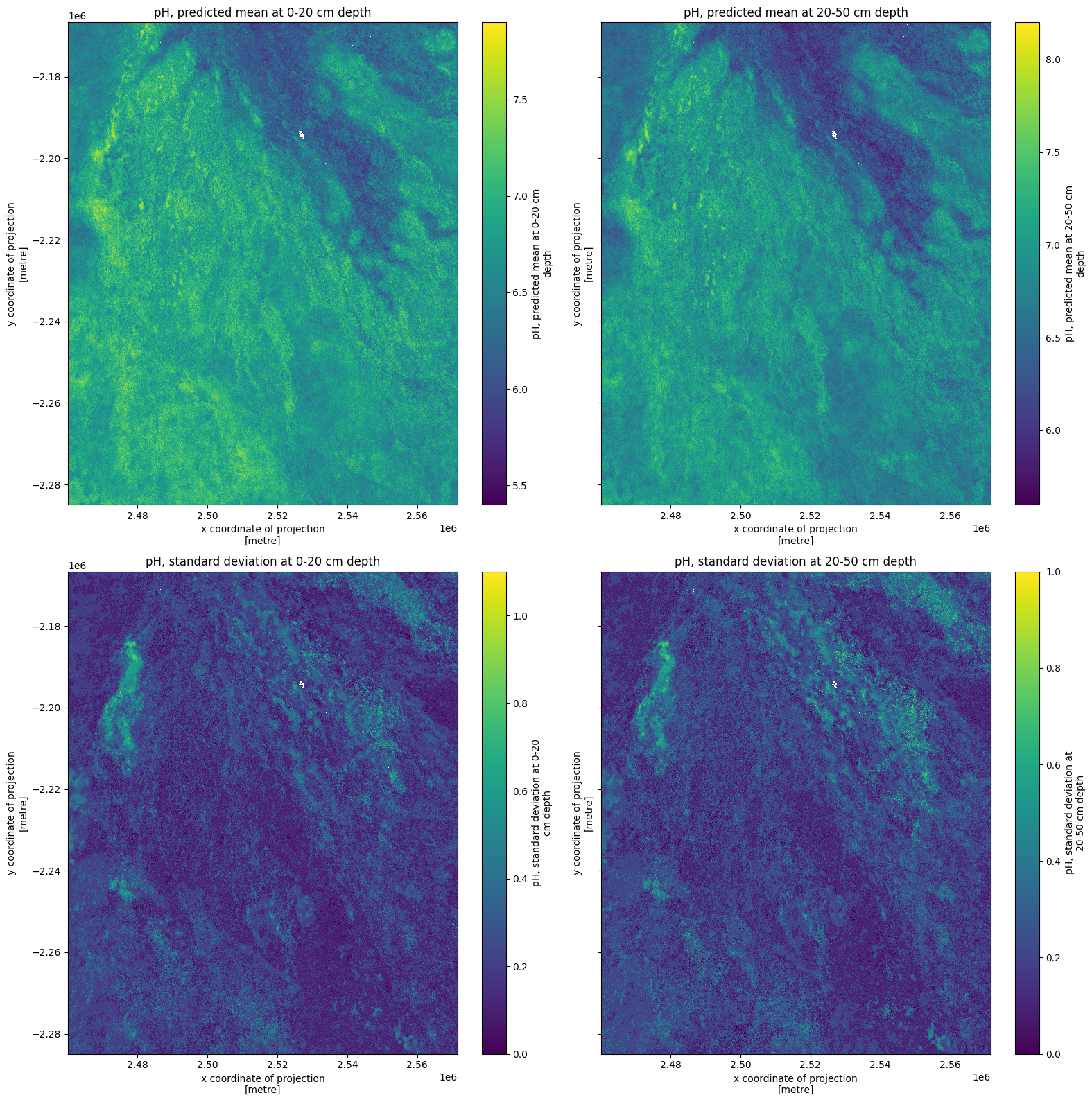
pH du sol

Enfin, nous inspecterons le pH du sol pour la même région du delta de l’Okavango.

Les définitions « lat » et « lon » resteront constantes, seul le « var » est modifié ci-dessous, conformément au tableau avec les noms d’accès au début du bloc-notes.

var = 'ph'

ds = load_isda(var, (lat-buffer, lat + buffer), (lon-buffer, lon + buffer))
ds

/usr/local/lib/python3.10/dist-packages/rioxarray/_io.py:430: NodataShadowWarning: The dataset's nodata attribute is shadowing the alpha band. All masks will be determined by the nodata attribute
  out = riods.read(band_key, window=window, masked=self.masked)
/usr/local/lib/python3.10/dist-packages/rioxarray/_io.py:430: NodataShadowWarning: The dataset's nodata attribute is shadowing the alpha band. All masks will be determined by the nodata attribute
  out = riods.read(band_key, window=window, masked=self.masked)
/usr/local/lib/python3.10/dist-packages/rioxarray/_io.py:430: NodataShadowWarning: The dataset's nodata attribute is shadowing the alpha band. All masks will be determined by the nodata attribute
  out = riods.read(band_key, window=window, masked=self.masked)
/usr/local/lib/python3.10/dist-packages/rioxarray/_io.py:430: NodataShadowWarning: The dataset's nodata attribute is shadowing the alpha band. All masks will be determined by the nodata attribute
  out = riods.read(band_key, window=window, masked=self.masked)

<xarray.Dataset>
Dimensions:                                   (x: 3711, y: 3940)
Coordinates:
  * x                                         (x) float64 2.46e+06 ... 2.571e+06
  * y                                         (y) float64 -2.167e+06 ... -2.2...
    spatial_ref                               int64 0
    band                                      <U9 'band_data'
Data variables:
    pH, predicted mean at 0-20 cm depth       (y, x) float32 65.0 65.0 ... 66.0
    pH, predicted mean at 20-50 cm depth      (y, x) float32 66.0 65.0 ... 67.0
    pH, standard deviation at 0-20 cm depth   (y, x) float32 1.0 1.0 ... 2.0 1.0
    pH, standard deviation at 20-50 cm depth  (y, x) float32 1.0 1.0 ... 1.0 1.0

xarray.Dataset

• Dimensions:
  • x: 3711
  • y: 3940
• Coordinates: (4)
  • x
    (x)
    float64
    2.46e+06 2.46e+06 ... 2.571e+06

    axis :

    X

    long_name :

    x coordinate of projection

    standard_name :

    projection_x_coordinate

    units :

    metre

    array([2460172.192357, 2460202.192357, 2460232.192357, ..., 2571412.192357,
           2571442.192357, 2571472.192357])

  • y
    (y)
    float64
    -2.167e+06 ... -2.285e+06

    axis :

    Y

    long_name :

    y coordinate of projection

    standard_name :

    projection_y_coordinate

    units :

    metre

    array([-2166721.869548, -2166751.869548, -2166781.869548, ..., -2284831.869548,
           -2284861.869548, -2284891.869548])

  • spatial_ref
    ()
    int64
    0

    crs_wkt :

    PROJCS["WGS 84 / Pseudo-Mercator",GEOGCS["WGS 84",DATUM["WGS_1984",SPHEROID["WGS 84",6378137,298.257223563,AUTHORITY["EPSG","7030"]],AUTHORITY["EPSG","6326"]],PRIMEM["Greenwich",0,AUTHORITY["EPSG","8901"]],UNIT["degree",0.0174532925199433,AUTHORITY["EPSG","9122"]],AUTHORITY["EPSG","4326"]],PROJECTION["Mercator_1SP"],PARAMETER["central_meridian",0],PARAMETER["scale_factor",1],PARAMETER["false_easting",0],PARAMETER["false_northing",0],UNIT["metre",1,AUTHORITY["EPSG","9001"]],AXIS["Easting",EAST],AXIS["Northing",NORTH],EXTENSION["PROJ4","+proj=merc +a=6378137 +b=6378137 +lat_ts=0 +lon_0=0 +x_0=0 +y_0=0 +k=1 +units=m +nadgrids=@null +wktext +no_defs"],AUTHORITY["EPSG","3857"]]

    spatial_ref :

    PROJCS["WGS 84 / Pseudo-Mercator",GEOGCS["WGS 84",DATUM["WGS_1984",SPHEROID["WGS 84",6378137,298.257223563,AUTHORITY["EPSG","7030"]],AUTHORITY["EPSG","6326"]],PRIMEM["Greenwich",0,AUTHORITY["EPSG","8901"]],UNIT["degree",0.0174532925199433,AUTHORITY["EPSG","9122"]],AUTHORITY["EPSG","4326"]],PROJECTION["Mercator_1SP"],PARAMETER["central_meridian",0],PARAMETER["scale_factor",1],PARAMETER["false_easting",0],PARAMETER["false_northing",0],UNIT["metre",1,AUTHORITY["EPSG","9001"]],AXIS["Easting",EAST],AXIS["Northing",NORTH],EXTENSION["PROJ4","+proj=merc +a=6378137 +b=6378137 +lat_ts=0 +lon_0=0 +x_0=0 +y_0=0 +k=1 +units=m +nadgrids=@null +wktext +no_defs"],AUTHORITY["EPSG","3857"]]

    GeoTransform :

    2460157.1923569688 30.0 0.0 -2166706.86954757 0.0 -30.0

    array(0)

  • band
    ()
    <U9
    'band_data'

    array('band_data', dtype='<U9')

• Data variables: (4)
  • pH, predicted mean at 0-20 cm depth
    (y, x)
    float32
    65.0 65.0 65.0 ... 65.0 67.0 66.0

    array([[65., 65., 65., ..., 61., 62., 61.],
           [65., 65., 65., ..., 61., 62., 62.],
           [65., 65., 66., ..., 61., 61., 61.],
           ...,
           [70., 71., 71., ..., 66., 66., 66.],
           [71., 71., 70., ..., 65., 66., 66.],
           [73., 70., 71., ..., 65., 67., 66.]], dtype=float32)

  • pH, predicted mean at 20-50 cm depth
    (y, x)
    float32
    66.0 65.0 66.0 ... 67.0 68.0 67.0

    array([[66., 65., 66., ..., 62., 63., 62.],
           [65., 66., 66., ..., 61., 62., 62.],
           [66., 66., 67., ..., 61., 60., 60.],
           ...,
           [71., 72., 72., ..., 67., 67., 68.],
           [72., 72., 72., ..., 66., 67., 67.],
           [74., 72., 72., ..., 67., 68., 67.]], dtype=float32)

  • pH, standard deviation at 0-20 cm depth
    (y, x)
    float32
    1.0 1.0 1.0 1.0 ... 1.0 1.0 2.0 1.0

    array([[1., 1., 1., ..., 2., 1., 2.],
           [1., 1., 1., ..., 2., 2., 2.],
           [1., 1., 1., ..., 2., 2., 2.],
           ...,
           [2., 4., 3., ..., 1., 1., 2.],
           [3., 4., 3., ..., 1., 1., 1.],
           [6., 3., 3., ..., 1., 2., 1.]], dtype=float32)

  • pH, standard deviation at 20-50 cm depth
    (y, x)
    float32
    1.0 1.0 1.0 1.0 ... 1.0 1.0 1.0 1.0

    array([[1., 1., 1., ..., 2., 2., 2.],
           [1., 1., 1., ..., 2., 2., 2.],
           [1., 1., 1., ..., 2., 2., 3.],
           ...,
           [2., 3., 3., ..., 1., 1., 1.],
           [3., 3., 3., ..., 1., 1., 1.],
           [5., 3., 3., ..., 1., 1., 1.]], dtype=float32)

• Indexes: (2)
  • x
    PandasIndex

    PandasIndex(Index([2460172.1923569688, 2460202.1923569688, 2460232.1923569688,
           2460262.1923569688, 2460292.1923569688, 2460322.1923569688,
           2460352.1923569688, 2460382.1923569688, 2460412.1923569688,
           2460442.1923569688,
           ...
           2571202.1923569688, 2571232.1923569688, 2571262.1923569688,
           2571292.1923569688, 2571322.1923569688, 2571352.1923569688,
           2571382.1923569688, 2571412.1923569688, 2571442.1923569688,
           2571472.1923569688],
          dtype='float64', name='x', length=3711))

  • y
    PandasIndex

    PandasIndex(Index([-2166721.86954757, -2166751.86954757, -2166781.86954757,
           -2166811.86954757, -2166841.86954757, -2166871.86954757,
           -2166901.86954757, -2166931.86954757, -2166961.86954757,
           -2166991.86954757,
           ...
           -2284621.86954757, -2284651.86954757, -2284681.86954757,
           -2284711.86954757, -2284741.86954757, -2284771.86954757,
           -2284801.86954757, -2284831.86954757, -2284861.86954757,
           -2284891.86954757],
          dtype='float64', name='y', length=3940))

• Attributes: (0)

Appliquer la transformation

Vérifiez si et comment les données doivent être transformées.

conversion = assets[var].extra_fields["back-transformation"]
conversion

'x/10'

Nous devons diviser par 10, ce qui est exécuté ci-dessous.

L’inspection du xarray.Dataset ci-dessus, à partir du moment où nous avons appelé « ds », indique également la nécessité d’une transformation. Nous nous attendrions à ce que les valeurs de pH soient comprises entre 0 et 14, mais nous pouvons voir des valeurs autour de 60-70. La plage ci-dessous, après division par 10, semble meilleure.

ds = ds / 10
ds

<xarray.Dataset>
Dimensions:                                   (x: 3711, y: 3940)
Coordinates:
  * x                                         (x) float64 2.46e+06 ... 2.571e+06
  * y                                         (y) float64 -2.167e+06 ... -2.2...
    spatial_ref                               int64 0
    band                                      <U9 'band_data'
Data variables:
    pH, predicted mean at 0-20 cm depth       (y, x) float32 6.5 6.5 ... 6.7 6.6
    pH, predicted mean at 20-50 cm depth      (y, x) float32 6.6 6.5 ... 6.8 6.7
    pH, standard deviation at 0-20 cm depth   (y, x) float32 0.1 0.1 ... 0.2 0.1
    pH, standard deviation at 20-50 cm depth  (y, x) float32 0.1 0.1 ... 0.1 0.1

xarray.Dataset

• Dimensions:
  • x: 3711
  • y: 3940
• Coordinates: (4)
  • x
    (x)
    float64
    2.46e+06 2.46e+06 ... 2.571e+06

    axis :

    X

    long_name :

    x coordinate of projection

    standard_name :

    projection_x_coordinate

    units :

    metre

    array([2460172.192357, 2460202.192357, 2460232.192357, ..., 2571412.192357,
           2571442.192357, 2571472.192357])

  • y
    (y)
    float64
    -2.167e+06 ... -2.285e+06

    axis :

    Y

    long_name :

    y coordinate of projection

    standard_name :

    projection_y_coordinate

    units :

    metre

    array([-2166721.869548, -2166751.869548, -2166781.869548, ..., -2284831.869548,
           -2284861.869548, -2284891.869548])

  • spatial_ref
    ()
    int64
    0

    crs_wkt :

    PROJCS["WGS 84 / Pseudo-Mercator",GEOGCS["WGS 84",DATUM["WGS_1984",SPHEROID["WGS 84",6378137,298.257223563,AUTHORITY["EPSG","7030"]],AUTHORITY["EPSG","6326"]],PRIMEM["Greenwich",0,AUTHORITY["EPSG","8901"]],UNIT["degree",0.0174532925199433,AUTHORITY["EPSG","9122"]],AUTHORITY["EPSG","4326"]],PROJECTION["Mercator_1SP"],PARAMETER["central_meridian",0],PARAMETER["scale_factor",1],PARAMETER["false_easting",0],PARAMETER["false_northing",0],UNIT["metre",1,AUTHORITY["EPSG","9001"]],AXIS["Easting",EAST],AXIS["Northing",NORTH],EXTENSION["PROJ4","+proj=merc +a=6378137 +b=6378137 +lat_ts=0 +lon_0=0 +x_0=0 +y_0=0 +k=1 +units=m +nadgrids=@null +wktext +no_defs"],AUTHORITY["EPSG","3857"]]

    spatial_ref :

    PROJCS["WGS 84 / Pseudo-Mercator",GEOGCS["WGS 84",DATUM["WGS_1984",SPHEROID["WGS 84",6378137,298.257223563,AUTHORITY["EPSG","7030"]],AUTHORITY["EPSG","6326"]],PRIMEM["Greenwich",0,AUTHORITY["EPSG","8901"]],UNIT["degree",0.0174532925199433,AUTHORITY["EPSG","9122"]],AUTHORITY["EPSG","4326"]],PROJECTION["Mercator_1SP"],PARAMETER["central_meridian",0],PARAMETER["scale_factor",1],PARAMETER["false_easting",0],PARAMETER["false_northing",0],UNIT["metre",1,AUTHORITY["EPSG","9001"]],AXIS["Easting",EAST],AXIS["Northing",NORTH],EXTENSION["PROJ4","+proj=merc +a=6378137 +b=6378137 +lat_ts=0 +lon_0=0 +x_0=0 +y_0=0 +k=1 +units=m +nadgrids=@null +wktext +no_defs"],AUTHORITY["EPSG","3857"]]

    GeoTransform :

    2460157.1923569688 30.0 0.0 -2166706.86954757 0.0 -30.0

    array(0)

  • band
    ()
    <U9
    'band_data'

    array('band_data', dtype='<U9')

• Data variables: (4)
  • pH, predicted mean at 0-20 cm depth
    (y, x)
    float32
    6.5 6.5 6.5 6.5 ... 6.6 6.5 6.7 6.6

    array([[6.5, 6.5, 6.5, ..., 6.1, 6.2, 6.1],
           [6.5, 6.5, 6.5, ..., 6.1, 6.2, 6.2],
           [6.5, 6.5, 6.6, ..., 6.1, 6.1, 6.1],
           ...,
           [7. , 7.1, 7.1, ..., 6.6, 6.6, 6.6],
           [7.1, 7.1, 7. , ..., 6.5, 6.6, 6.6],
           [7.3, 7. , 7.1, ..., 6.5, 6.7, 6.6]], dtype=float32)

  • pH, predicted mean at 20-50 cm depth
    (y, x)
    float32
    6.6 6.5 6.6 6.5 ... 6.7 6.7 6.8 6.7

    array([[6.6, 6.5, 6.6, ..., 6.2, 6.3, 6.2],
           [6.5, 6.6, 6.6, ..., 6.1, 6.2, 6.2],
           [6.6, 6.6, 6.7, ..., 6.1, 6. , 6. ],
           ...,
           [7.1, 7.2, 7.2, ..., 6.7, 6.7, 6.8],
           [7.2, 7.2, 7.2, ..., 6.6, 6.7, 6.7],
           [7.4, 7.2, 7.2, ..., 6.7, 6.8, 6.7]], dtype=float32)

  • pH, standard deviation at 0-20 cm depth
    (y, x)
    float32
    0.1 0.1 0.1 0.1 ... 0.1 0.1 0.2 0.1

    array([[0.1, 0.1, 0.1, ..., 0.2, 0.1, 0.2],
           [0.1, 0.1, 0.1, ..., 0.2, 0.2, 0.2],
           [0.1, 0.1, 0.1, ..., 0.2, 0.2, 0.2],
           ...,
           [0.2, 0.4, 0.3, ..., 0.1, 0.1, 0.2],
           [0.3, 0.4, 0.3, ..., 0.1, 0.1, 0.1],
           [0.6, 0.3, 0.3, ..., 0.1, 0.2, 0.1]], dtype=float32)

  • pH, standard deviation at 20-50 cm depth
    (y, x)
    float32
    0.1 0.1 0.1 0.1 ... 0.1 0.1 0.1 0.1

    array([[0.1, 0.1, 0.1, ..., 0.2, 0.2, 0.2],
           [0.1, 0.1, 0.1, ..., 0.2, 0.2, 0.2],
           [0.1, 0.1, 0.1, ..., 0.2, 0.2, 0.3],
           ...,
           [0.2, 0.3, 0.3, ..., 0.1, 0.1, 0.1],
           [0.3, 0.3, 0.3, ..., 0.1, 0.1, 0.1],
           [0.5, 0.3, 0.3, ..., 0.1, 0.1, 0.1]], dtype=float32)

• Indexes: (2)
  • x
    PandasIndex

    PandasIndex(Index([2460172.1923569688, 2460202.1923569688, 2460232.1923569688,
           2460262.1923569688, 2460292.1923569688, 2460322.1923569688,
           2460352.1923569688, 2460382.1923569688, 2460412.1923569688,
           2460442.1923569688,
           ...
           2571202.1923569688, 2571232.1923569688, 2571262.1923569688,
           2571292.1923569688, 2571322.1923569688, 2571352.1923569688,
           2571382.1923569688, 2571412.1923569688, 2571442.1923569688,
           2571472.1923569688],
          dtype='float64', name='x', length=3711))

  • y
    PandasIndex

    PandasIndex(Index([-2166721.86954757, -2166751.86954757, -2166781.86954757,
           -2166811.86954757, -2166841.86954757, -2166871.86954757,
           -2166901.86954757, -2166931.86954757, -2166961.86954757,
           -2166991.86954757,
           ...
           -2284621.86954757, -2284651.86954757, -2284681.86954757,
           -2284711.86954757, -2284741.86954757, -2284771.86954757,
           -2284801.86954757, -2284831.86954757, -2284861.86954757,
           -2284891.86954757],
          dtype='float64', name='y', length=3940))

• Attributes: (0)

fig, ax = plt.subplots(2, 2, figsize=(16, 16), sharey=True)
ds[list(ds.keys())[0]].plot(ax=ax[0, 0])
ds[list(ds.keys())[1]].plot(ax=ax[0, 1])
ds[list(ds.keys())[2]].plot(ax=ax[1, 0])
ds[list(ds.keys())[3]].plot(ax=ax[1, 1])
ax[0, 0].set_title(list(ds.keys())[0])
ax[0, 1].set_title(list(ds.keys())[1])
ax[1, 0].set_title(list(ds.keys())[2])
ax[1, 1].set_title(list(ds.keys())[3])
plt.tight_layout();

Conclusions

Ce carnet a donné une introduction au chargement des données de sol iSDA dans le bac à sable de Digital Earth Africa.

Existe-t-il des modèles observables entre la formation du delta de l’Okavango, la teneur en argile et le pH du sol ? Comment la carte de classification de la capacité de fertilité correspond-elle à l’image en vraies couleurs ?

Ce carnet est destiné à servir de point de départ. Les utilisateurs peuvent essayer de charger des données pour d’autres zones ou d’autres variables du sol.

---

Informations Complémentaires

Licence : Le code de ce carnet est sous licence Apache, version 2.0 <https://www.apache.org/licenses/LICENSE-2.0>. Les données de Digital Earth Africa sont sous licence Creative Commons par attribution 4.0 <https://creativecommons.org/licenses/by/4.0/>.

Contact : Si vous avez besoin d’aide, veuillez poster une question sur le canal Slack Open Data Cube <http://slack.opendatacube.org/>`__ ou sur le GIS Stack Exchange en utilisant la balise open-data-cube (vous pouvez consulter les questions posées précédemment ici). Si vous souhaitez signaler un problème avec ce bloc-notes, vous pouvez en déposer un sur Github.

Version de Datacube compatible :

print(datacube.__version__)

1.8.15

Dernier test :

from datetime import datetime
datetime.today().strftime('%Y-%m-%d')

'2023-08-11'