L’empreinte de la colonisation mondiale (WSF)
Mots-clés: données utilisées ; Empreinte de peuplement mondial, ensembles de données ; wsf_2015 ensembles de données ; wsf_2019 données utilisées ; Empreinte de peuplement mondial
Aperçu
Selon le Département des affaires économiques et sociales de l’ONU, la planète comptera 9,7 milliards d’habitants d’ici 2050. 55 % de la population mondiale réside actuellement dans des zones urbaines et ce chiffre devrait atteindre 68 % d’ici 2050. L’urbanisation rapide et anarchique, associée aux problèmes posés par le changement climatique, peut accroître la pollution de l’air, rendre les populations plus vulnérables aux catastrophes et entraîner des problèmes de gestion des ressources telles que l’eau, les matières premières et l’énergie (Mapping Our Human Footprint From Space, 2023).
Afin d’améliorer la compréhension des tendances actuelles de l’urbanisation mondiale, l’ESA et le Centre aérospatial allemand (DLR), en collaboration avec l’équipe de Google Earth Engine, développent conjointement l’empreinte mondiale des établissements humains – l’ensemble de données le plus complet au monde sur les établissements humains (G.D.Team, 2023).
L”empreinte mondiale de peuplement 2015 est un masque binaire d’une résolution de 10 m (0,32 seconde d’arc) décrivant l’étendue de la colonisation mondiale de 2015, dérivée de l’exploitation conjointe du radar multitemporel Sentinel-1 et de l’imagerie satellite optique Landsat-8 (Marconcini et al., 2020).
L”Empreinte mondiale des établissements humains 2019 présente les données des missions Copernicus Sentinel-1 et Sentinel-2 et fournit des informations sur les établissements humains mondiaux avec un niveau de détail et une précision sans précédent (Marconcini et al., 2021).
Les données de l’Empreinte Mondiale des Établissements 2015 et 2019 sont désormais indexées dans la plateforme DE Africa.
Description
Ce bloc-notes est une procédure pas à pas sur la façon d’utiliser l’empreinte de peuplement mondial 2015 et 2019 dans le cube de données. L’exemple pratique guide les utilisateurs à travers le code requis pour :
Inspecter l’ensemble de données WSF
Utilisez la fonction « dc.load() » pour charger le jeu de données WSF
Résultats du tracé pour l’ensemble de données WSF ***
Commencer
Pour exécuter cette analyse, exécutez toutes les cellules du bloc-notes, en commençant par la cellule « Charger les packages ».
Charger des paquets
[1]:
%matplotlib inline

import datacube
import numpy as np
import pandas as pd
import geopandas as gpd
import seaborn as sns

import matplotlib.pyplot as plt
import matplotlib.ticker as mticker
from matplotlib.colors import ListedColormap
from matplotlib.patches import Patch
import matplotlib.animation as animation
from mpl_toolkits.axes_grid1 import make_axes_locatable
from IPython.display import Image
from odc.geo.geom import Geometry

from deafrica_tools.plotting import display_map
from deafrica_tools.areaofinterest import define_area
Se connecter au datacube
[2]:
dc = datacube.Datacube(app="wsf")
Liste des mesures
Nous pouvons inspecter les données disponibles pour le WSF en utilisant la fonctionnalité « list_measurements » de datacube. Le tableau ci-dessous répertorie les produits et mesures disponibles pour les trois jeux de données WSF indexés dans le datacube de DE Africa.
[3]:
product_name = ['wsf_2015', 'wsf_2019']

dc_measurements = dc.list_measurements()
dc_measurements.loc[product_name].drop('flags_definition', axis=1)
[3]:
| name | dtype | units | nodata | aliases | scale_factor | ||
|---|---|---|---|---|---|---|---|
| product | measurement | ||||||
| wsf_2015 | wsf2015 | wsf2015 | uint8 | 1 | 0.0 | [wsf2015] | NaN |
| wsf_2019 | wsf2019 | wsf2019 | uint8 | 1 | 0.0 | [wsf2019] | NaN |
Paramètres d’analyse
Pour définir la zone d’intérêt, deux méthodes sont disponibles :
En spécifiant la latitude, la longitude et la zone tampon. Cette méthode nécessite que vous saisissiez la latitude centrale, la longitude centrale et la valeur de la zone tampon en degrés carrés autour du point central que vous souhaitez analyser. Par exemple, « lat = 10,338 », « lon = -1,055 » et « buffer = 0,1 » sélectionneront une zone avec un rayon de 0,1 degré carré autour du point avec les coordonnées (10,338, -1,055).
By uploading a polygon as a
GeoJSON or Esri Shapefile. If you choose this option, you will need to upload the geojson or ESRI shapefile into the Sandbox using Upload Files button in the top left corner of the Jupyter Notebook interface. ESRI shapefiles must be uploaded with all the related files
 (.cpg, .dbf, .shp, .shx). Once uploaded, you can use the shapefile or geojson to define the area of interest. Remember to update the code to call the file you have uploaded.
Pour utiliser l’une de ces méthodes, vous pouvez décommenter la ligne de code concernée et commenter l’autre. Pour commenter une ligne, ajoutez le symbole "#" avant le code que vous souhaitez commenter. Par défaut, la première option qui définit l’emplacement à l’aide de la latitude, de la longitude et du tampon est utilisée.
L’emplacement par défaut est Kumasi, région Ashanti, Ghana
[4]:
# Method 1: Specify the latitude, longitude, and buffer
aoi = define_area(lat= 6.69856, lon=-1.62331, buffer=0.2)

# Method 2: Use a polygon as a GeoJSON or Esri Shapefile.
#aoi = define_area(vector_path='aoi.shp')

#Create a geopolygon and geodataframe of the area of interest
geopolygon = Geometry(aoi["features"][0]["geometry"], crs="epsg:4326")
geopolygon_gdf = gpd.GeoDataFrame(geometry=[geopolygon], crs=geopolygon.crs)

# Get the latitude and longitude range of the geopolygon
lat_range = (geopolygon_gdf.total_bounds[1], geopolygon_gdf.total_bounds[3])
lon_range = (geopolygon_gdf.total_bounds[0], geopolygon_gdf.total_bounds[2])

# defining the color scheme for wfs 2015 and 2019 plotting
ft_2015 = '#D3D3D3'
ft_2019 = '#e5ab00'
Afficher l’emplacement sélectionné
La cellule suivante affichera la zone sélectionnée sur une carte interactive. N’hésitez pas à zoomer et dézoomer pour mieux comprendre la zone que vous allez analyser. En cliquant sur n’importe quel point de la carte, vous découvrirez les coordonnées de latitude et de longitude de ce point.
[5]:
display_map(x=lon_range, y=lat_range)
[5]:
Chargement du jeu de données WSF
L’ensemble de données WSF sera chargé à l’aide de la fonction « dc.load ». Pour plus d’informations sur la manière de charger des données à l’aide du datacube, reportez-vous au bloc-notes « Introduction au chargement des données <../Beginners_guide/03_Loading_data.ipynb> »__.
La cellule ci-dessous charge l’ensemble de données wsf_2015. Notez les valeurs « produit » et « mesures ». Celles-ci seront mises à jour pour les données suivantes lors de leur chargement.
[6]:
#create reusable datacube query object
query = {
    'x': lon_range,
    'y': lat_range,
    'resolution':(-10, 10),
    'output_crs': 'epsg:6933',
}

#load the data and save it in wsf_2015 variable
wsf_2015 = dc.load(product='wsf_2015', measurements ='wsf2015', **query).squeeze()

#print out results
display(wsf_2015)
<xarray.Dataset> Size: 20MB
Dimensions:      (y: 5070, x: 3860)
Coordinates:
    time         datetime64[ns] 8B 2015-07-02T11:59:59.500000
  * y            (y) float64 41kB 8.78e+05 8.78e+05 ... 8.273e+05 8.273e+05
  * x            (x) float64 31kB -1.759e+05 -1.759e+05 ... -1.373e+05
    spatial_ref  int32 4B 6933
Data variables:
    wsf2015      (y, x) uint8 20MB 0 0 0 0 0 0 0 0 0 0 0 ... 0 0 0 0 0 0 0 0 0 0
Attributes:
    crs:           epsg:6933
grid_mapping: spatial_refLa cellule ci-dessous charge l’ensemble de données wsf_2019, notez que le produit et la mesure sont respectivement modifiés en « wsf_2019 » et « wsf2019 ». À part cela, la requête est la même que la requête précédente définie.
[7]:
wsf_2019 = dc.load(product='wsf_2019',
                 measurements='wsf2019',
                 **query).squeeze()

display(wsf_2019)
<xarray.Dataset> Size: 20MB
Dimensions:      (y: 5070, x: 3860)
Coordinates:
    time         datetime64[ns] 8B 2019-07-02T11:59:59.500000
  * y            (y) float64 41kB 8.78e+05 8.78e+05 ... 8.273e+05 8.273e+05
  * x            (x) float64 31kB -1.759e+05 -1.759e+05 ... -1.373e+05
    spatial_ref  int32 4B 6933
Data variables:
    wsf2019      (y, x) uint8 20MB 0 0 0 0 0 0 0 0 0 0 0 ... 0 0 0 0 0 0 0 0 0 0
Attributes:
    crs:           epsg:6933
grid_mapping: spatial_refTracé spatial des données
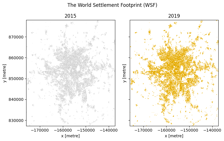
L’ensemble de données WSF est fourni avec deux valeurs de pixels : « 0 » (aucune donnée) et « 255 » (empreinte de peuplement). Pour le graphique ci-dessous, comme nous sommes intéressés par l’empreinte de peuplement, l’ensemble de données sera filtré pour n’inclure que les valeurs « 255 ». Après le filtrage, les ensembles de données WSF pour 2015 et 2019 sont représentés.
[8]:
# storing datsets in the wsf_2015
wsf_2015 = wsf_2015.wsf2015

# storing datsets in the wsf_2019
wsf_2019 = wsf_2019.wsf2019

#Plotting of Dataset
fig, ax = plt.subplots(1, 2, figsize=(8, 5), sharey=True)

#filtering of the 2015 for only the 255 values
wsf_2015.where(wsf_2015 == 255).plot(ax=ax[0], add_colorbar=False,cmap=ListedColormap([ft_2015]))

#filtering of the 2019 for only the 255 values
wsf_2019.where(wsf_2015 == 255).plot(ax=ax[1], add_colorbar=False,cmap=ListedColormap([ft_2019]))
ax[0].set_title("2015")
ax[1].set_title("2019")
plt.suptitle('The World Settlement Footprint (WSF)')
plt.tight_layout()
plt.show();
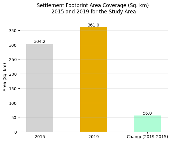
Calculer la surface de l’empreinte de la colonie
Le nombre de pixels peut être utilisé pour la surface du bâtiment si la surface en pixels est connue. Exécutez la cellule suivante pour générer les constantes nécessaires à la réalisation de cette conversion.
[9]:
pixel_length = query["resolution"][1]  # in metres
m_per_km = 1000  # conversion from metres to kilometres
area_per_pixel = pixel_length**2 / m_per_km**2
La valeur constante « area_per_pixel » calculée ci-dessus sera multipliée par le nombre de pixels pour obtenir la superficie de l’empreinte du bâtiment pour 2015 et 2019. La superficie sera tracée dans un graphique à barres pour comparer les valeurs métriques à travers l’évolution des bâtiments entre les deux années.
[10]:
# Calculating the area for 2015
wsf_2015_area = wsf_2015.where(wsf_2015 == 255).count() * area_per_pixel

#Calculating the area for 2015
wsf_2019_area = wsf_2019.where(wsf_2019 == 255).count() * area_per_pixel

#Calculating the area for difference between 2015 and 2019
wsf_diff = (wsf_2019_area - wsf_2015_area)

fig, ax = plt.subplots()
bar_plot = ax.bar(x = ['2015', '2019', 'Change(2019-2015)'], height = [wsf_2015_area, wsf_2019_area, wsf_diff],
       color=[ft_2015,ft_2019, '#aefcd5'], width=0.5)

ax.bar_label(bar_plot, fmt=lambda x: '{:.1f}'.format(x))

ax.set_ylabel("Area (Sq. km)")
ax.set_title(f"Settlement Footprint Area Coverage (Sq. km) \n 2015 and 2019 for the Study Area \n")
ax.grid(axis='y', linewidth=0.3)
ax.spines['right'].set_visible(False)
ax.spines['top'].set_visible(False)

plt.show()
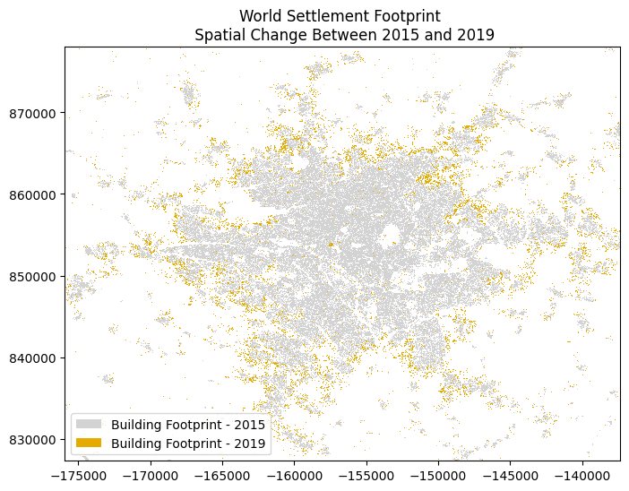
Tracé des changements spatiaux
Un graphique à barres a permis de visualiser la comparaison de la zone de peuplement entre 2015 et 2019, mais un tracé spatial nous permettra de visualiser les zones où il y a eu un développement de peuplement. Pour identifier les zones qui ont connu un changement entre 2015 et 2019, 2015 servira de référence par rapport à 2019. La différence sera représentée graphiquement pour déterminer la zone de changement.
[11]:
wsf_change =  wsf_2015.where(wsf_2015 == 255, 0) - wsf_2019.where(wsf_2019 == 255, 0)

wsf_2015.where(wsf_2015 == 255).plot.imshow(cmap=ListedColormap([ft_2015]),
                                               add_colorbar=False, add_labels=False,
                                               figsize=(8,6))

wsf_change.where(wsf_change == 1).plot.imshow(cmap=ListedColormap([ft_2019]),
                           add_colorbar=False, add_labels=False)

plt.legend(
        [Patch(facecolor=ft_2015), Patch(facecolor=ft_2019)],
        ['Building Footprint - 2015', 'Building Footprint - 2019'],
         loc = 'lower left');

plt.title('World Settlement Footprint \n Spatial Change Between 2015 and 2019');

plt.show()
Conclusion
L’Empreinte Mondiale des Établissements offre une base de connaissances qui peut aider les chercheurs, les organisations gouvernementales et d’autres parties prenantes, telles que les urbanistes, à mieux comprendre comment l’urbanisation se produit et, simultanément, à mettre en place des stratégies de développement urbain durable pour des décisions politiques éclairées aux niveaux local et national.
Note
Pour exécuter une zone différente, accédez à la cellule Paramètres d’analyse, modifiez les valeurs lat et lon dans define_area_function.
Référencement
Cartographie de notre empreinte humaine depuis l’espace (consulté en août 2023). ESA - Cartographie de notre empreinte humaine depuis l’espace. https://www.esa.int/Applications/Observing_the_Earth/Mapping_our_human_footprint_from_space
Marconcini, M., Metz-Marconcini, A., Üreyen, S. et al. Décrire les lieux de vie des humains, l’empreinte mondiale des peuplements 2015. Sci Data 7, 242 (2020). https://doi.org/10.1038/s41597-020-00580-5
Mattia Marconcini, Annekatrin Metz-Marconcini, Thomas Esch et Noel Gorelick. Comprendre les tendances actuelles de l’urbanisation mondiale - The World Settlement Footprint Suite. GI_Forum 2021, numéro 1, 33-38 (2021) https://austriaca.at/0xc1aa5576%200x003c9b4c.pdf
G.D.Team (consulté en août 2023). Contextes cartographiques des géoservices de l’EOC. Contextes cartographiques des géoservices de l’EOC. https://geoservice.dlr.de/web/maps
Informations Complémentaires
Licence : Le code de ce carnet est sous licence Apache, version 2.0 <https://www.apache.org/licenses/LICENSE-2.0>. Les données de Digital Earth Africa sont sous licence Creative Commons par attribution 4.0 <https://creativecommons.org/licenses/by/4.0/>.
Contact : Si vous avez besoin d’aide, veuillez poster une question sur le canal Slack Open Data Cube <http://slack.opendatacube.org/>`__ ou sur le GIS Stack Exchange en utilisant la balise open-data-cube (vous pouvez consulter les questions posées précédemment ici). Si vous souhaitez signaler un problème avec ce bloc-notes, vous pouvez en déposer un sur Github.
Version de Datacube compatible :
[12]:
print(datacube.__version__)
1.8.20
Dernier test :
[13]:
from datetime import datetime
datetime.today().strftime('%Y-%m-%d')
[13]:
'2025-01-15'