GeoMAD cloud-free composites

Date modified: March 2022

Service overview

Background

GeoMAD is the Digital Earth Africa (DE Africa) surface reflectance geomedian and triple Median Absolute Deviation data service. It is a cloud-free composite of satellite data compiled over specific timeframes. This service is ideal for:

• Longer-term time series analysis

• Cloud-free imagery

• Statistical accuracy

GeoMAD has two main components:

• Geomedian

• Median Absolute Deviations (MADs)

The geomedian component combines measurements collected over the specified timeframe to produce one representative, multispectral measurement for every pixel unit of the African continent. The end result is a comprehensive dataset that can be used to generate true-colour images for visual inspection of anthropogenic or natural landmarks. The full spectral dataset can be used to develop more complex algorithms.

For each pixel, invalid data is discarded, and the remaining observations are mathematically summarised using the geomedian statistic. Flyover coverage provided by collecting data over a period of time also helps scope intermittently cloudy areas.

Variations between the geomedian and the individual measurements are captured by the three Median Absolute Deviation (MAD) layers. These are higher-order statistical measurements calculating variation relative to the geomedian. The MAD layers can be used on their own or together with geomedian to gain insights about the land surface, and understand change over time.

Calculating GeoMAD over different timeframes and sensors provides a range of insights to the environment. An annual timeframe allows better correction for cloud cover and reduces artifacts for comparison over multiple years. A shorter timeframe, for example, six-month or three-month blocks, better captures seasonal variation within one year, and can be used to compare equivalent periods from different years. Landsat sensors allow full utility of the surface reflectance archive dating back to 1984, while more recent Sentinel-2 data provides higher-frequency flyovers and better resolution.

The Digital Earth Africa GeoMAD service currently provides annual, six-month semiannual and rolling monthly (3-month moving window) datasets, with separate services for Landsat and Sentinel-2 sensors.

Jupyter Notebooks that demonstrate loading and using GeoMAD and Rolling GeoMAD datasets in the Sandbox are also available.

Specifications

The GeoMAD service spans all of Africa and is currently available in three timeframes:

• Annual: observations from one calendar year are summarised into one set of measurements

  • Sentinel-2 Annual GeoMAD

  • Landsat 8 Annual GeoMAD

  • Landsat 5 & 7 Annual GeoMAD

  • Landsat 8 & 9 Annual GeoMAD

• Semiannual: observations are summarised for each half of the calendar year, giving one set of measurements for January–June, and one for July–December

  • Sentinel-2 Semiannual GeoMAD

• Rolling GeoMAD: observations are summarised over rolling three-month periods starting on the first day of each calendar month, giving a set of new measurements each month e.g Jan-Mar, Feb-Apr, Mar-May and so on.

  • Sentinel-2 Rolling Monthly GeoMAD

GeoMAD metadata can also be viewed on Digital Earth Africa’s Metadata Explorer.

Table 1: Sentinel-2 GeoMAD service specifications

Specification
Service name	Sentinel-2 Annual GeoMAD	Sentinel-2 Semiannual GeoMAD	Sentinel-2 Rolling Monthly GeoMAD
Service status	Operational	Operational	Operational
Number of bands	14	14	14
Cell size - X (metres)	10	10	10
Cell size - Y (metres)	10	10	10
Coordinate reference system (CRS)	EPSG: 6933	EPSG: 6933	EPSG: 6933
Temporal resolution	Annual	6-monthly (Jan-Jun, Jul-Dec)	Monthly (3-month rolling window)
Temporal range	2017 – current	2017 – current	2019 – current
Parent dataset	Sentinel-2 Level-2A	Sentinel-2 Level-2A	Sentinel-2 Level-2A
Update frequency	Annual	6 months	Monthly
Update latency	2 months from end of previous year	2 months from end of previous half year	1 month from end of previous period

Table 2: Landsat GeoMAD service specifications

Specification
Service name	Landsat 8 & 9 Annual GeoMAD	Landsat 8 Annual GeoMAD	Landsat 5 & 7 Annual GeoMAD
Service status	Operational	Operational	Operational
Number of bands	10	10	10
Cell size - X (metres)	30	30	30
Cell size - Y (metres)	30	30	30
Coordinate reference system (CRS)	EPSG: 6933	EPSG: 6933	EPSG: 6933
Temporal resolution	Annual	Annual	Annual
Temporal range	2021 –	2013 – 2020	1984 – 2012
Parent dataset	Landsat Level-2 Collection 2	Landsat Level-2 Collection 2	Landsat Level-2 Collection 2
Update frequency	Annual	Annual	NA
Update latency	2 months from end of previous year	2 months from end of previous year	NA

The Landsat 5 & 7 Annual GeoMAD service combines data from both the Landsat 5 and Landsat 7 sensors. It is produced for the 1984 – 2012 archive only. Similarly, the Landsat 8 & 9 Annual GeoMAD came into production after Landsat 9 data became available in late 2021.

Figure 1: GeoMAD geographic extent

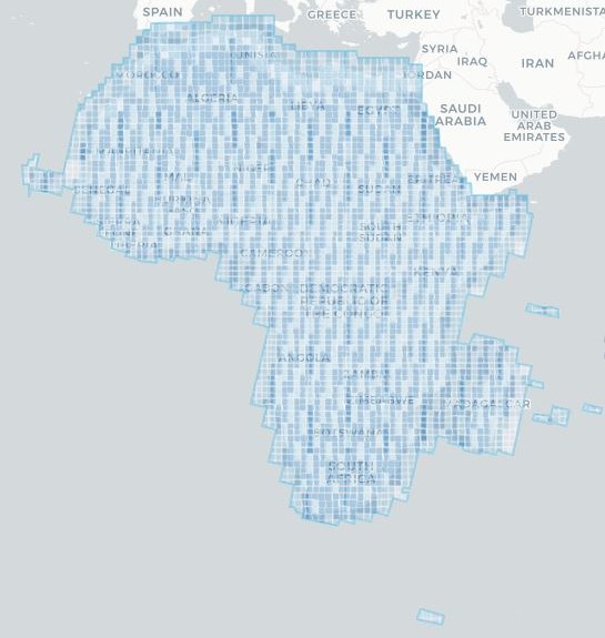
Digital Earth Africa GeoMAD data is available for the regions shaded in blue. Specific temporal and geographic extents can be explored as an interactive map on the Digital Earth Africa Metadata Explorer.

Sentinel-2, Landsat 8, and Landsat 8 & 9 GeoMAD services are generated from parent datasets with frequent satellite flyovers consistent with the geographic extent shown in Figure 1. While the Landsat 5 & Landsat 7 Annual GeoMAD also covers the same area, there are some limitations associated with the sparsity of the Landsat archive over Africa, particularly before the launch of Landsat 7 in 1999.

This is visually displayed in the count imagery in Figure 2. Northern and southern Africa have the best coverage over the archive period. Central and western Africa show lower data counts, and therefore less years where a geomedian and MADs have been calculated. It is recommended to consult the Digital Earth Africa Metadata Explorer for precise data availability of the Landsat 5 and 7 GeoMAD.

Figure 2: Landsat 5 & 7 GeoMAD data extent

Left: An animation showing data count over Africa for the years 1984 to 2012. Darker blue indicates higher counts, while lighter blue is lower counts. Areas with very low or zero counts in one year do not have enough data to calculate a geomedian or MADs for that year.

Right: A static image showing the number of years for which a geomedian has been calculated. In the 29 years between 1984 and 2012, northern and southern Africa show almost complete geomedian coverage, while central and western Africa have a lower geomedian count associated with less data acquisition over the time period.

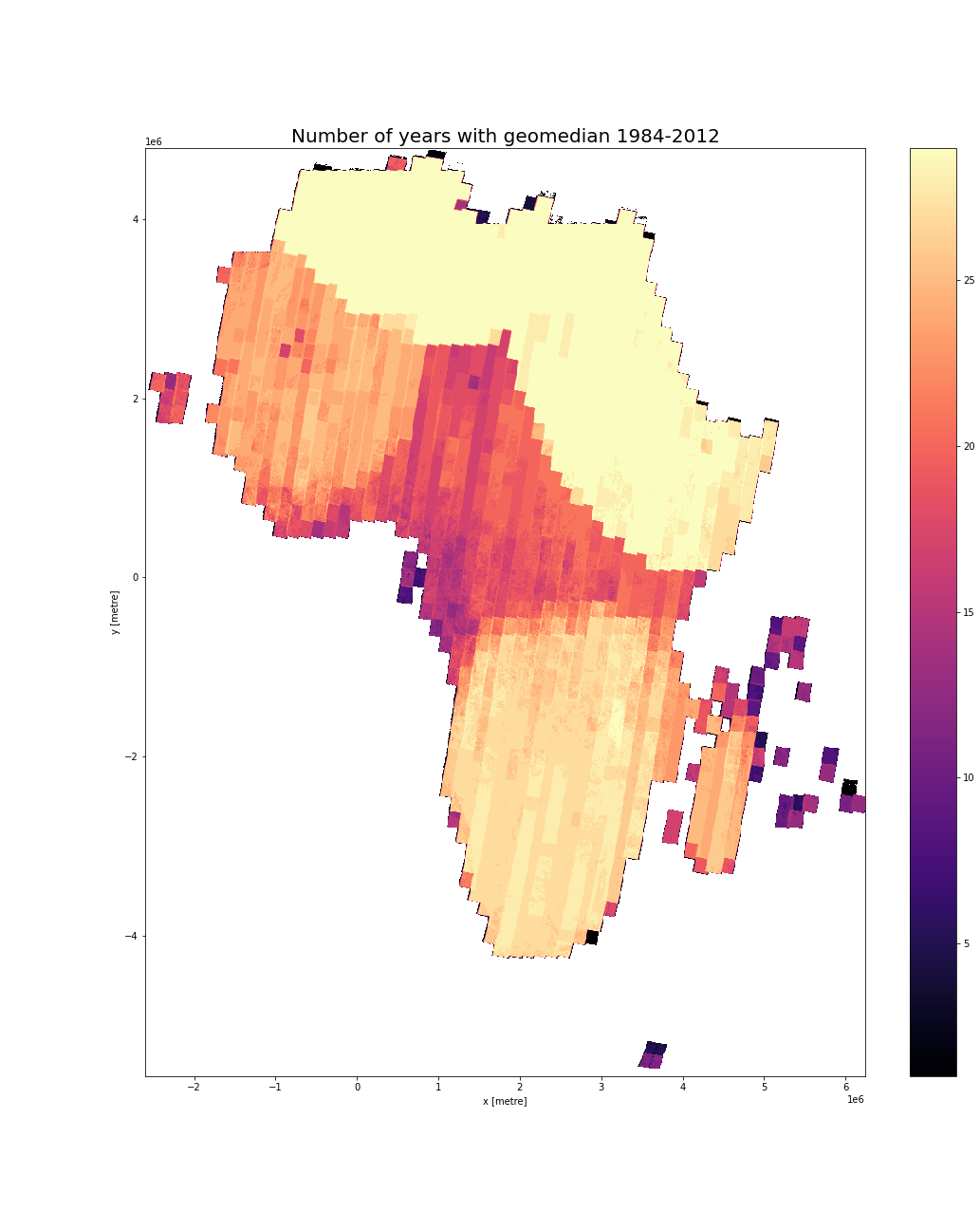
Table 3.1: Sentinel-2 GeoMAD measurements

Band ID	Description	Value range	Data type	No data value
B02	Geomedian B02 (Blue)	1 - 10000	uint16	0
B03	Geomedian B03 (Green)	1 - 10000	uint16	0
B04	Geomedian B04 (Red)	1 - 10000	uint16	0
B05	Geomedian B05 (Red edge 1)	1 - 10000	uint16	0
B06	Geomedian B06 (Red edge 2)	1 - 10000	uint16	0
B07	Geomedian B07 (Red edge 3)	1 - 10000	uint16	0
B08	Geomedian B08 (Near infrared (NIR) 1)	1 - 10000	uint16	0
B8A	Geomedian B8A (NIR 2)	1 - 10000	uint16	0
B11	Geomedian B11 (Short-wave infrared (SWIR) 1)	1 - 10000	uint16	0
B12	Geomedian B12 (SWIR 2)	1 - 10000	uint16	0
SMAD	Spectral Median Absolute Deviation	0 - 1	float32	NaN
EMAD	Euclidean Median Absolute Deviation	0 - 31623	float32	NaN
BCMAD	Bray-Curtis Median Absolute Deviation	0 - 1	float32	NaN
COUNT	Number of clear observations	1 - 65535	uint16	0

Table 3.2: Landsat 8 and Landsat 8 & 9 GeoMAD measurements

Band ID	Description	Value range	Data type	No data value
SR_B2	Geomedian SR_B2 (Blue)	1 - 10000	uint16	0
SR_B3	Geomedian SR_B3 (Green)	1 - 10000	uint16	0
SR_B4	Geomedian SR_B4 (Red)	1 - 10000	uint16	0
SR_B5	Geomedian SR_B5 (NIR)	1 - 10000	uint16	0
SR_B6	Geomedian SR_B6 (SWIR 1)	1 - 10000	uint16	0
SR_B7	Geomedian SR_B7 (SWIR 2)	1 - 10000	uint16	0
SMAD	Spectral Median Absolute Deviation	0 - 1	float32	NaN
EMAD	Euclidean Median Absolute Deviation	0 - 31623	float32	NaN
BCMAD	Bray-Curtis Median Absolute Deviation	0 - 1	float32	NaN
COUNT	Number of clear observations	1 - 65535	uint16	0

Table 3.3: Landsat 5 & Landsat 7 GeoMAD measurements

Band ID	Description	Value range	Data type	No data value
SR_B1	Geomedian SR_B1 (Blue)	1 - 10000	uint16	0
SR_B2	Geomedian SR_B2 (Green)	1 - 10000	uint16	0
SR_B3	Geomedian SR_B3 (Red)	1 - 10000	uint16	0
SR_B4	Geomedian SR_B4 (NIR)	1 - 10000	uint16	0
SR_B5	Geomedian SR_B5 (SWIR 1)	1 - 10000	uint16	0
SR_B7	Geomedian SR_B7 (SWIR 2)	1 - 10000	uint16	0
SMAD	Spectral Median Absolute Deviation	0 - 1	float32	NaN
EMAD	Euclidean Median Absolute Deviation	0 - 31623	float32	NaN
BCMAD	Bray-Curtis Median Absolute Deviation	0 - 1	float32	NaN
COUNT	Number of clear observations	1 - 65535	uint16	0

Bands can be subdivided as follows:

• Geomedian - 10 bands (Sentinel-2), 6 bands (Landsat 5/7/8/9): The geomedian is calculated using the spectral bands of data collected during the specified time period. Surface reflectance values have been scaled between 1 and 10000 to allow for more efficient data storage as unsigned 16-bit integers (uint16). Note parent datasets often contain more bands, some of which are not used in GeoMAD.

The geomedian band IDs correspond to bands in the parent Sentinel-2 Level-2A data. For example, the Annual GeoMAD band B02 contains the annual geomedian of the Sentinel-2 B02 band.

• Median Absolute Deviations (MADs) - 3 bands: Deviations from the geomedian are quantified through median absolute deviation calculations. The GeoMAD service utilises three MADs, each stored in a separate band: Euclidean MAD (EMAD), spectral MAD (SMAD), and Bray-Curtis MAD (BCMAD). Each MAD is calculated using the same ten bands as in the geomedian. SMAD and BCMAD are normalised ratios, therefore they are unitless and their values always fall between 0 and 1. EMAD is a function of surface reflectance but is neither a ratio nor normalised, therefore its valid value range depends on the number of bands used in the geomedian calculation - ten in GeoMAD.

• Count - 1 band: The number of clear satellite measurements of a pixel for that calendar year. This is around 60 for Sentinel-2 and 20 for Landsat 8 annually, but doubles at areas of overlap between scenes. “Count” is not incorporated in either the geomedian or MADs calculations. It is intended for metadata analysis and data validation.

Processing

All clear observations for the given time period are collated from the parent dataset. Cloudy pixels are identified and excluded. The geomedian and MADs calculations are then performed by the hdstats package.

Media and example images

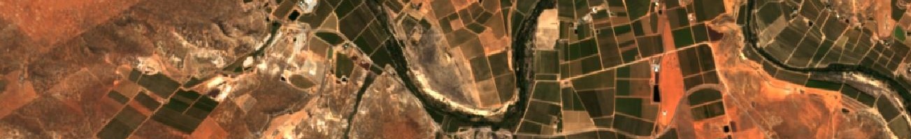
Image 1: Animations over northern Africa. 1984 – 2012 Landsat 5 & 7 Annual geomedian, true-colour (RGB).

Left: Agricultural area expansion near Sadat City, Egypt.

Right: Urbanisation in Tangier, Morocco.

Credit: Contains Landsat Level-2 Surface Reflectance Science Product courtesy of the U.S. Geological Survey, processed by Digital Earth Africa.

Image 2: Mangroves in Guinea-Bissau. 2019 Sentinel-2 Annual geomedian, true-colour (RGB).

Credit: Contains modified Copernicus Sentinel data 2019, processed by Digital Earth Africa.

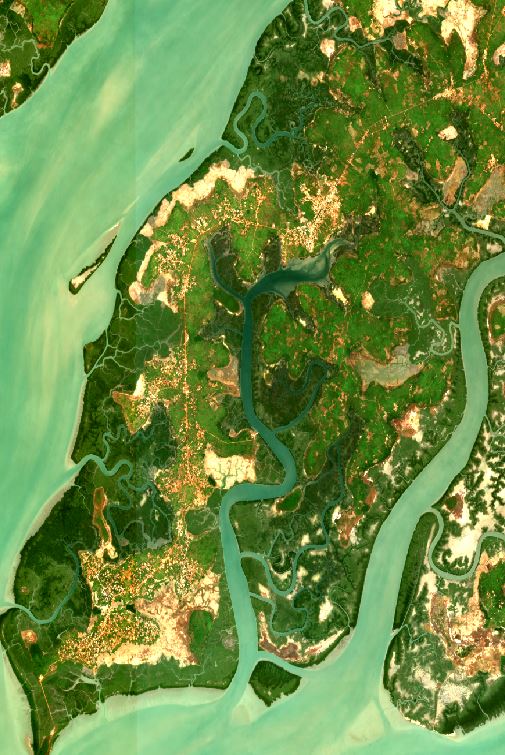
Image 3: Croplands in South Africa. 2019 Sentinel-2 Annual triple MADs, plotted as RGB.

Credit: Contains modified Copernicus Sentinel data 2019, processed by Digital Earth Africa.

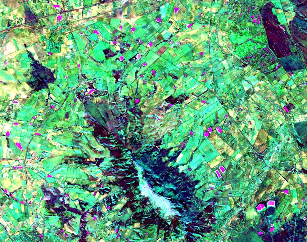
Image 4: Irrigated fields in Egypt. Jan-Jun 2020 (right), Jul-Dec 2020 (left). 2020 Sentinel-2 Semiannual geomedian, true-colour (RGB).

Credit: Contains modified Copernicus Sentinel data 2020, processed by Digital Earth Africa.

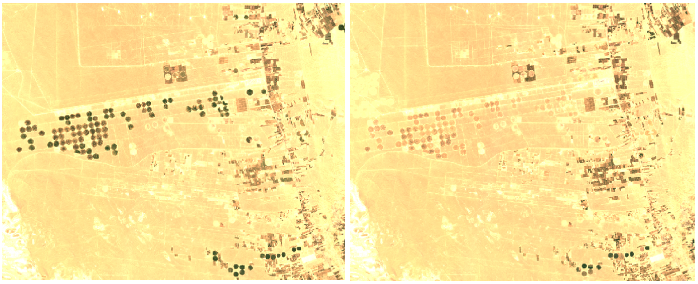
Image 5: The Okavango Delta, Botswana. 2020 Landsat 8 Annual triple MADs, plotted as RGB.

Credit: Contains Landsat Level-2 Surface Reflectance Science Product courtesy of the U.S. Geological Survey, processed by Digital Earth Africa.

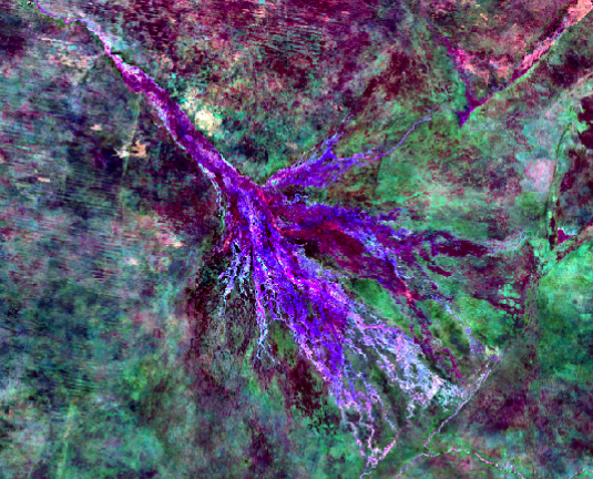
Image 6: Animations 2020–2022 using Sentinel-2 Rolling GeoMAD, true-colour (RGB)

The dates shown are the midpoints of the Rolling GeoMAD.

Credit: Contains modified Copernicus Sentinel data 2022, processed by Digital Earth Africa.

Farmland in northern Egypt

Wetland in Guinea Bissua

Known limitations

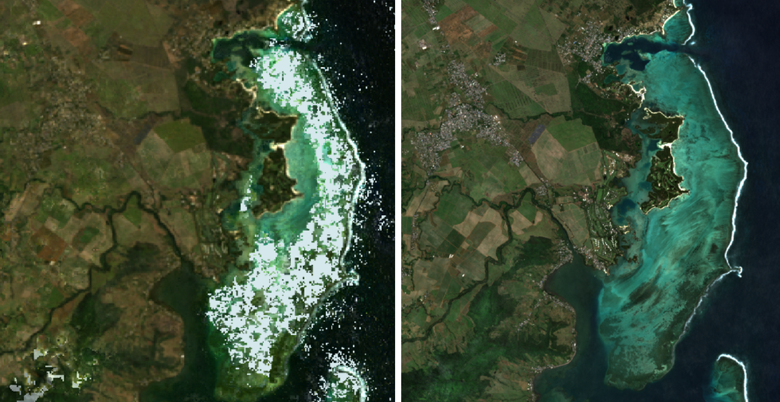
The Landsat 8 (& 9) GeoMAD has a known issue with data quality over marine regions. The GeoMAD algorithm uses pixel quality information from the input data to identify and mask pixels with poor quality obervations. Landsat 8 & 9 analysis ready satellite images over the ocean often contain negative surface reflectance values, and the GeoMAD masking procedures remove pixels where any negative values occur. Thus, in regions where pixels are persistently negative throughout the year, the GeoMAD product will contain a no-data value. An example of this can be seen in Image 7 below where a shallow marine system contains no-data values in the GeoMAD because the NIR band values in the input data are persistently negative.

Image 7: Shallow marine system, Mauritius. 2021 Landsat 8 Annual GeoMAD (left), versus Sentinel-2 GeoMAD (right), plotted as RGB.

Maps portal link

Related services

• Sentinel-2 Level-2A Surface Reflectance

• Landsat Collection 2 Level-2 Surface Reflectance

References

Roberts, D., Mueller, N., & Mcintyre, A. (2017). High-dimensional pixel composites from Earth observation time series. IEEE Transactions on Geoscience and Remote Sensing, 55(11), 6254-6264. https://doi.org/10.1109/TGRS.2017.2723896

Roberts, D., Dunn, B., Mueller, N. (2018). Open Data Cube products using high-dimensional statistics of time series. 8647-8650. https://doi.org/10.1109/IGARSS.2018.8518312.

License

CC BY Attribution 4.0 International License

Acknowledgements

The high-dimensional statistics algorithms incorporated in this service are the work of Dr Dale Roberts, Australian National University.

Data access

Amazon Web Services S3

GeoMAD data can be accessed from the associated S3 bucket.

Table 3: AWS data access details

AWS S3 details
Bucket ARN	arn:aws:s3:::deafrica-services
Product name	gm_s2_annual, gm_ls8_annual, gm_ls5_ls7_annual, gm_s2_semiannual, gm_s2_rolling

The bucket is in the AWS region af-south-1 (Cape Town). Additional region specifications can be applied as follows:

aws s3 ls --region=af-south-1 s3://deafrica-services/gm_s2_annual/

The file paths follow the format:

<productname>/<version>/<x>/<y>/<timeperiod>/<x><y>_<timeperiod>_<band>.<extension>

Table 4: AWS file path convention

File path element	Description	Example
productname	Product name	gm_s2_annual
version	Product version	1.0.0
x	Tile number in the x direction.	x17
y	Tile number in the y direction.	y156
timeperiod	Year of data collection followed by period of time and time unit in the format YYYY--P<period><unit>. Time units are designated by capitalised letters, Y for years and M for months. Annual data is P1Y while 6-monthly data (such as the semiannuals) is P6M.	2019--P1Y
x_y_timeperiod_band.extension	File name. Combines x, y, timeperiod with band, using Band IDs, and file extensions. For most tiles, the file extension is .tif.

Tile numbering uses 96 km grid squares based on the default CRS for this product, EPSG:6933, with the origin set at the bottom-leftmost corner of the valid EPSG:6933 region.

OGC Web Services (OWS)

This service is available through DE Africa’s OWS.

Table 5: OWS data access details

OWS details
Name	DE Africa Services
Web Map Services (WMS) URL	https://ows.digitalearth.africa/wms?version=1.3.0
Web Coverage Service (WCS) URL	https://ows.digitalearth.africa/wcs?version=2.1.0
Layer name	gm_s2_annual, gm_ls8_annual, gm_ls5_ls7_annual, gm_s2_semiannual

Digital Earth Africa OWS details can be found at https://ows.digitalearth.africa/.

For instructions on how to connect to OWS, see this tutorial.

Open Data Cube (ODC)

GeoMAD datasets are accessible in the Digital Earth Africa ODC API, which is available through the Digital Earth Africa Sandbox.

Specific bands of data can be called by using either the default names or any of a band’s alternative names, as listed in the table below. ODC datacube.Datacube.load commands without specified bands will load all bands; see ODC documentation.

Table 6.1: Sentinel-2 GeoMAD ODC product and band names

ODC product name: gm_s2_annual, gm_s2_semiannual, gm_s2_rolling

Band name	Alternative names
B02	band_02, blue
B03	band_03, green
B04	band_04, red
B05	band_05, red_edge_1
B06	band_06, red_edge_2
B07	band_07, red_edge_3
B08	band_08, nir, nir_1
B8A	band_8a, nir_narrow, nir_2
B11	band_11, swir_1, swir_16
B12	band_12, swir_2, swir_22
SMAD	smad, sdev, SDEV
EMAD	emad, edev, EDEV
BCMAD	bcmad, bcdev, BCDEV
COUNT	count

Table 6.2: Landsat 8 GeoMAD ODC product and band names

ODC product name: gm_ls8_annual

Band name	Alternative names
SR_B2	band_2, blue
SR_B3	band_3, green
SR_B4	band_4, red
SR_B5	band_5, nir
SR_B6	band_6, swir_1
SR_B7	band_7, swir_2
SMAD	smad, sdev, SDEV
EMAD	emad, edev, EDEV
BCMAD	bcmad, bcdev, BCDEV
COUNT	count

Table 6.3: Landsat 5 & 7 GeoMAD ODC product and band names

ODC product name: gm_ls5_ls7_annual

Band name	Alternative names
SR_B1	band_1, blue
SR_B2	band_2, green
SR_B3	band_3, red
SR_B4	band_4, nir
SR_B5	band_5, swir_1
SR_B7	band_7, swir_2
SMAD	smad, sdev, SDEV
EMAD	emad, edev, EDEV
BCMAD	bcmad, bcdev, BCDEV
COUNT	count

Product names and band names are case-sensitive.

For examples on how to use the ODC API, see the DE Africa example notebook repository.

Technical information

Geomedian

Pixel composites are created by compiling multiple satellite observations of the same area to form one representative image. They have become a staple to Earth observation research as combining measurements compensates for missing data, such as gaps caused by cloud cover. This results in comprehensive datasets that allow thorough analysis of large areas of interest.

There are many ways of forming this image. GeoMAD uses the geomedian summary statistic to combine six months or a year of data into one scientifically-rigorous composite. It produces one multispectral observation for each pixel on continental Africa.

The geomedian statistic is sometimes referred to as the “geometric median”, as in the figure below. To remove ambiguity with other kinds of statistics with similar names, it is always referred to in DE Africa as the “geomedian”.

Figure 2: Illustrated explanation of the geomedian.

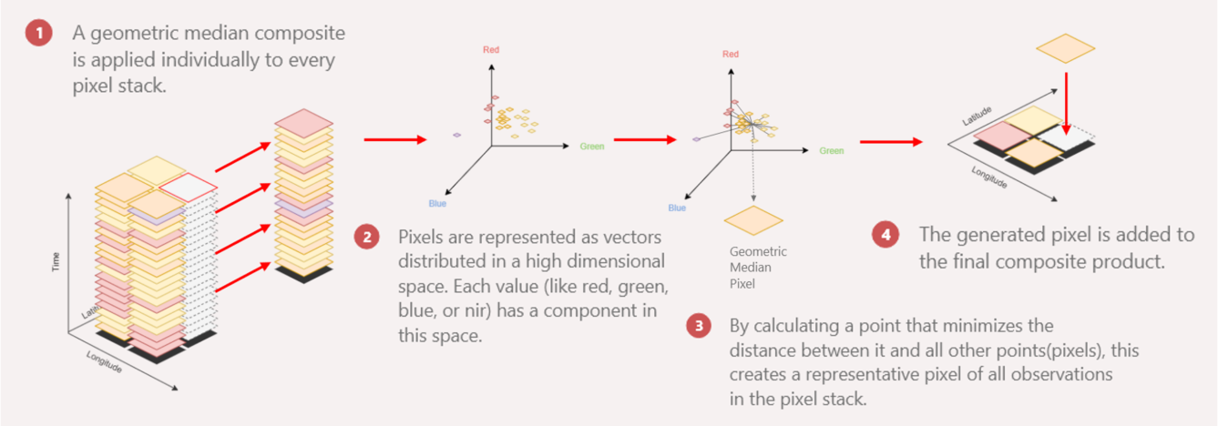
Figure 2 uses a three-dimensional example to illustrate how the geomedian is calculated for a single pixel containing multiple measurements of red, blue and green data.

• The dataset has \(N\) timesteps of satellite data. In the case of Figure 2, \(N=20\)

• Each timestep contains \(p\) bands. In this case, \(p =3\) (one dimension each for red, green, blue)

• Therefore each timestep can be represented by a 3-dimensional vector \(\mathbf{x}\). A single vector at timestep \(t\), \(\mathbf{x}^{(t)}\), looks like this:

:nbsphinx-math:`begin{align*} mathbf{x}^{(t)} = begin{bmatrix}

x^{(t)}_{red} \ x^{(t)}_{green}\ x^{(t)}_{blue}

end{bmatrix} end{align*}`

• The entire dataset can be represented as the collection of the vectors at every timestep \(\mathbf{x}^{(1)}, \mathbf{x}^{(2)}, \dots \mathbf{x}^{(20)}\)

Projected onto a plane, it will look like the plot in Figure 2.2 - twenty points placed depending on their values of red, green and blue. The geomedian of this pixel is then the point where the Euclidean distance (straight-line distance) between all data points is minimised. This is depicted in Figure 2.3; for further information on Euclidean distance, see the section below on the Euclidean MAD.

Let’s call the geomedian point in this example \(\mathbf{m}_\text{example}\). Euclidean distance between a point \(\mathbf{x}\) and the data points \(\mathbf{x}^{(t)}\) is given by \(\lVert \mathbf{x} - \mathbf{x}^{(t)} \rVert\). The point at which all twenty distances are minimised is found by taking the \(\mathrm{argmin}\); the argument of the minima. The geomedian can then be expressed by the following equation:

\begin{align*} \mathbf{m}_\text{example} = \underset{\mathbf{x} \in \mathbb{R}^3}{\mathrm{argmin}} \sum^{20}_{t=1} \lVert \mathbf{x} - \mathbf{x}^{(t)} \rVert \end{align*}

In this example, the resulting \(\mathbf{m}_\text{example}\), like any \(\mathbf{x}\), will be a 3-dimensional vector, with a value each for red, green, and blue.

:nbsphinx-math:`begin{align*} mathbf{m}_text{example} =begin{bmatrix}

m_{red} \ m_{green}\ m_{blue}

end{bmatrix} end{align*}`

The geomedian point \(\mathbf{m}\) is not selected from one of the twenty data points. It is a separate vector with unique values that do not necessarily correspond to existing band values from the observation dataset.

The formula for the geomedian of a single pixel can be generalised for \(p\) bands and \(N\) timesteps, as given in Roberts et al, 2017:

\begin{align*} \mathbf{m} = \underset{\mathbf{x} \in \mathbb{R}^p}{\mathrm{argmin}} \sum^{N}_{t=1} \lVert \mathbf{x} - \mathbf{x}^{(t)} \rVert \end{align*}

In the Sentinel-2 GeoMADs, the ten bands of the geomedian result in a 10-dimensional space - in the Landsat GeoMADs, the six geomedian bands give a 6-dimensional space. It is difficult to illustrate this example in six (or ten!) dimensions, but we can instead provide the equation, and the form of the result. Here, the number of timesteps \(N\) varies per pixel; pixels on the overlap between satellite swathes may have very large \(N\) (up to around 140 per year for Sentinel-2 annual services), while pixels in the centre of the path are only observed once per flyover, and have \(N\) closer to 70.

:nbsphinx-math:`begin{align*} mathbf{m}_text{GeoMAD} = underset{mathbf{x} in mathbb{R}^{10}}{mathrm{argmin}} sum^{N}_{t=1} lVert mathbf{x} - mathbf{x}^{(t)} rVert = begin{bmatrix}

m_{B02} \ m_{B03}\ m_{B04}\ m_{B05} \ m_{B06}\ m_{B07}\ m_{B08} \ m_{B8A}\ m_{B11}\ m_{B12}

end{bmatrix} end{align*}`

This calculation is repeated for every pixel in the specified extent.

The significance of the geomedian is that all bands are considered simultaneously. This maintains the spectral relationship between bands, providing the most representative value. Additionally, the geomedian statistic reduces spatial noise and improves colour balance compared to similar statistics such as the median or medoid.

The geomedian is therefore a vital foundational dataset for applications such as band index analysis on vegetation, water and urban area detection. It is also useful as a feature layer in machine learning algorithms.

DE Africa provides an interactive geomedian visualisation available as a Jupyter Notebook widget. It graphically compares the geomedian to a median for a 3-D example. An example screenshot is shown below.

Figure 3: Geomedian visualisation widget.

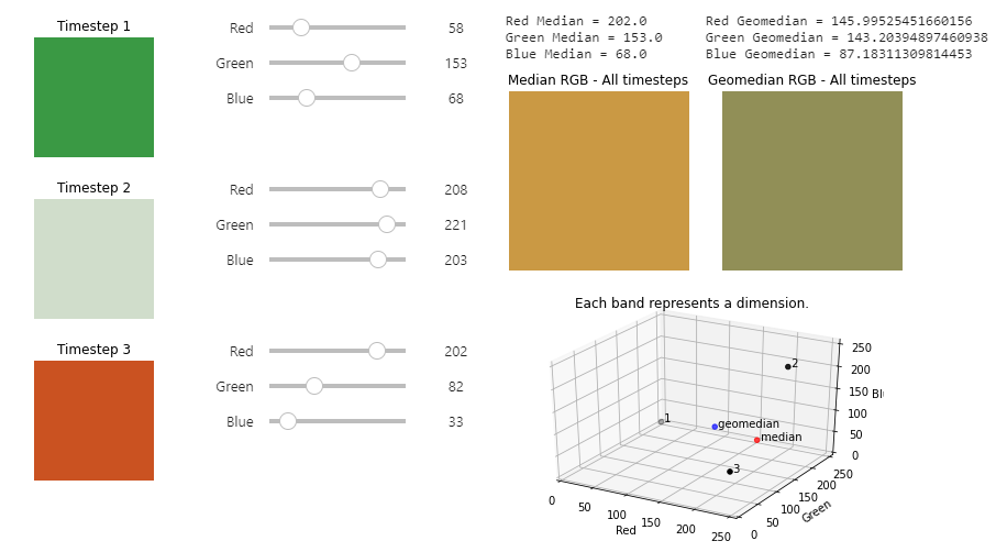
To interact with the widget, log in to the Digital Earth Africa Sandbox and navigate to the Datasets folder > GeoMAD.

Triple Median Absolute Deviations (MADs)

By definition, the geomedian smooths variations in the satellite data to pick the most central, representative value. Outlying extreme highs and lows are generally filtered out by the robustness of the geomedian calculation. However, it is still useful to know about the variation within the dataset. This results in a set of second-order statistics: the Median Absolute Deviations (MADs).

MADs are change statistics based on the geomedian. They show how much variation each pixel underwent in the given timeframe.

Let us break down the acronym “MAD”; as in the title, it stands for median absolute deviation:

• This implies we have a collection of measurements

• We then find the deviation of each measurement from a baseline value, obtaining one deviation for every measurement

• These deviations are all absolute values, so each deviation is equal to or greater than 0

• We then find the median, or middle value, of these deviations

• This gives us a median absolute deviation

In this case, our “collection of measurements” is satellite data from each flyover. Even for a single pixel, we have multiple measurements in the time axis: one from every pass.

The “baseline value” is the geomedian, which provides one multispectral result for each pixel.

The “deviations” here are three different distance or dissimilarity values. There are multiple ways of quantifying how change has occurred, so this service computes three different MADs for use in data analysis. We are calculating, in three separate ways, the deviation between the geomedian and a single flyover’s measurement. These three values have been chosen to reflect a range of changes that appear in Earth observation data, and hence this section of the dataset is often referred to as “triple MADs”.

The three MADs used in DE Africa are:

• Euclidean MAD, EMAD (based on Euclidean distance)

• Spectral MAD, SMAD (based on cosine distance)

• Bray-Curtis MAD, BCMAD (based on Bray-Curtis dissimilarity)

Each will be explained in their own sections below. Example calculations with real numbers are in the appendix.

Note there are many other types of statistical distances and dissimilarities that can be used for median absolute deviation analysis (for example: Manhattan distance, Canberra distance, there are many and they can all be used to calculate a MAD). However, in DE Africa services, the terms “triple MADs” or “MADs” are always specifically referring to the three MADs included in the GeoMAD dataset: EMAD, SMAD, and BCMAD.

Euclidean MAD (EMAD)

The most logical place to start thinking about any of the MADs is the Euclidean MAD (EMAD). This is because EMAD comes from Euclidean distance, and Euclidean distance can be explained with a physical analogy: it is how we measure straight-line distances between points. In our three-dimensional world, it may look like this:

Figure 4: Euclidean distance in three dimensions.

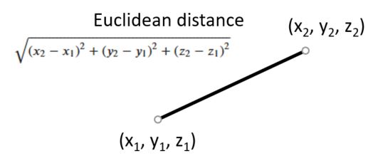
In the case of satellite data, we are measuring the Euclidean distance between a pixel’s geomedian value and a single multispectral measurement. The number of dimensions is equal to the number of bands in the data. In the illustration below, \(m\) is the geomedian value and \(\mathbf{x}\) the measured value. In real data, there will be multiple measurements over a time period, so \(t\) is the timestep number, otherwise noted in equations as superscript \((t)\).

For example, if we had three bands of data (red, green and blue), and three timesteps of data, then we can calculate the Euclidean distances as follows:

Figure 5: Euclidean distance in three dimensions over three timesteps.

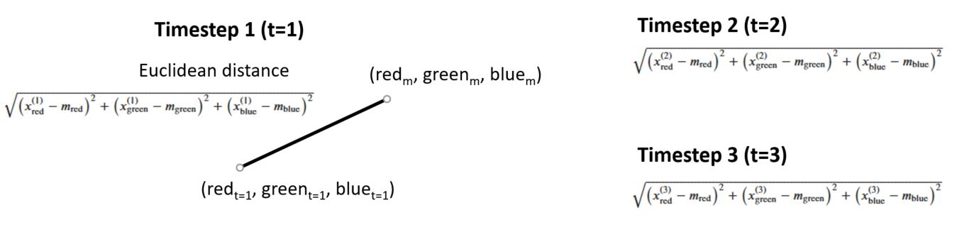
Each timestep gives a separate Euclidean distance result. Then EMAD is the median of all those distances.

In most real life conditions, there will be more than three timesteps and more than three bands. A general expression of Euclidean distance for \(p\) bands is given as:

\begin{align*} &\text{Multispectral Euclidean distance for timestep }t \\ =& \sqrt{ \left( x^{(t)}_{\text{band 1}} - m_{\text{band 1}} \right)^2 + \left( x^{(t)}_{\text{band 2}} - m_{\text{band 2}} \right)^2 + \dots + \left( x^{(t)}_{\text{band p}} - m_{\text{band p}} \right)^2 }\\ =& \lVert \mathbf{x}^{(t)} - m \rVert_{\mathbb{R}^p} \end{align*}

Then EMAD for \(N\) timesteps is given by Roberts et al, 2018, as the median of the Euclidean distances from all the timesteps.

\begin{align*} \text{EMAD} = \text{median} \left( \left\{ \lVert \mathbf{x}^{(t)} - \mathbf{m} \rVert_{\mathbb{R}^p}, t = 1, \dots , N \right\} \right) \end{align*}

In GeoMAD, the MADs are calculated from the same ten bands used in the geomedian, therefore \(p=10\). The result of \(\lVert \mathbf{x}^{(t)} - \mathbf{m} \rVert_{\mathbb{R}^p}\) is a positive scalar, so \(\text{EMAD}_\text{GeoMAD}\) is a positive scalar number. As in the geomedian, \(N\) is dependent on the number of satellite flyovers particular to that pixel.

\begin{align*} \text{EMAD}_\text{GeoMAD} = \text{median} \left( \left\{ \lVert \mathbf{x}^{(t)} - \mathbf{m} \rVert_{\mathbb{R}^{10}}, t = 1, \dots , N \right\} \right) \end{align*}

The maximum possible value for EMAD depends on the value ranges for each of the bands in the dataset. In the case of GeoMAD, which uses at maximum annual timescales of ten bands of Sentinel-2 data, valid EMAD values range from 0 - 31623.

EMAD is useful for showing albedo shifts in satellite spectra.

Spectral MAD (SMAD)

The spectral MAD (SMAD) is based on the median absolute deviations in the cosine distance between the geomedian and individual measurements.

In two dimensions, cosine distance can be graphically compared to Euclidean distance by the following figure:

Figure 6: Relative relationships between Euclidean and cosine distances.

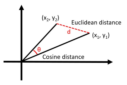
In a general sense, cosine distance is related to the angle between the two points \(\theta\), while Euclidean distance is related to the straight-line distance between the two points \(d\). Like Euclidean distance, points are more similar when the cosine distance between them is small. The value of the cosine distance is smaller when \(\theta\) is small (i.e. close to 0) or when \(\theta\) is close to 180\(^{\circ}\).

Notice we could have a small cosine distance but a large Euclidean distance; for example, if the angle between the vectors is small, but one is much longer than the other. This is an important property of cosine distance (and thus SMAD) - unlike Euclidean distance, cosine distance is not skewed by the magnitude of the measurements.

Cosine distance is defined more formally as:

\begin{align*} \text{Cosine distance (two dimensions)} = 1 - \frac{x_1 y_1 + x_2 y_2}{ \left( \sqrt{ \left( x_1\right) ^2 + \left( x_2\right) ^2 } \right) \left( \sqrt{ \left( y_1\right) ^2 + \left( y_2\right) ^2 } \right)} \end{align*}

For more than two dimensions, we can generalise the cosine distance formula for a single pixel. For a multispectral measurement of \(p\) bands at timestep \(t\), \(\mathbf{x}^{(t)}\), and the geomedian at the same point \(\mathbf{m}\), the cosine distance is:

\begin{align*}\small &\text{Multispectral cosdist}\left( \mathbf{x}^{(t)}, m \right) \text{ for timestep } t \\ &= 1 - \frac{ \mathbf{x}^{(t)} \cdot \mathbf{m} }{ \lVert \mathbf{x}^{(t)} \rVert \ \lVert \mathbf{m} \rVert} \ \text{ for } \mathbf{x}^{(t)}, \mathbf{m} \in \mathbb{R}_{p}\\ &= 1 - \left( \frac{\left( x_{\text{band 1}}^{(t)} \right) \left(m_{\text{band 1}} \right) + \left( x_{\text{band 2}}^{(t)} \right) \left(m_{\text{band 2}} \right) + \cdots + \left( x_{\text{band p}}^{(t)} \right) \left(m_{\text{band p}} \right)}{ \left(\sqrt{\left( x_{\text{band 1}}^{(t)} \right)^2 + \cdots+ \left( x_{\text{band p}}^{(t)} \right)^2} \right) \left( \sqrt{\left( m_{\text{band 1}} \right)^2 + \cdots+ \left( m_{\text{band p}} \right)^2 } \right)} \right) \end{align*}

Then for \(N\) timesteps, SMAD is the median of the cosine distances.

\begin{align*} \text{SMAD} = \text{median} \left( \left\{ \text{cosdist}\left( \mathbf{x}^{(t)}, \mathbf{m} \right), t = 1, \dots , N \right\} \right) \end{align*}

As with the other distances and dissimilarities used in the MADs, this results in a positive scalar value, thus SMAD is a positive scalar. Valid values for SMAD fall between 0 – 1.

In applications of Earth observation data, SMAD is useful for showing areas of land cover change. One reason is that SMAD is less affected by cloud; unlike EMAD, it is invariant to albedo changes, such as that caused by the diffusion of solar radiation. SMAD can also be used to track water bodies, as water has high variation in reflectance.

Bray-Curtis MAD (BCMAD)

The Bray-Curtis MAD (BCMAD) is calculated from the Bray-Curtis dissimilarity. The Bray-Curtis dissimilarity emphasises differences in each band between the measurement and the geomedian.

For a single band of satellite data, the Bray-Curtis dissimilarity looks remarkably like a normalised band index. For example, if we only had red band data, it might look something like this:

\begin{align*} \text{Single-band Bray-Curtis dissimilarity at timestep }t = \frac{\left| x_{\text{red}}^{(t)} - m_{\text{red}}\right|}{ \left| x_{\text{red}}^{(t)} + m_{\text{red}} \right| } \end{align*}

It can be generalised to a multispectral dataset with \(p\) bands:

\begin{align*} &\text{Multispectral Bray-Curtis dissimilarity for timestep }t\\ &= \frac{\left| x_{\text{band 1}}^{(t)} - m_{\text{band 1}}\right| + \left| x_{\text{band 2}}^{(t)} - m_{\text{band 2}} \right| + \dots + \left| x_{\text{band p}}^{(t)} - m_{\text{band p}} \right| }{ \left| x_{\text{band 1}}^{(t)} + m_{\text{band 1}} \right| + \left| x_{\text{band 2}}^{(t)} + m_{\text{band 2}} \right| + \dots + \left| x_{\text{band p}}^{(t)} + m_{\text{band p}} \right|} \end{align*}

The Bray-Curtis dissimilarity will be maximised at a value of 1 when the measurements in each band are completely different. Conversely, the value of the dissimilarity will be small where each band observation is similar to the geomedian of that band.

As with the other MADs, the BCMAD is found by taking the median of all the Bray-Curtis dissimilarities from \(N\) timesteps. For GeoMAD, \(p=10\).

\begin{align*} \text{BCMAD} = \text{median} \left( \left\{ \frac{\left| \mathbf{x}^{(t)} - \mathbf{m} \right|_{\mathbb{R}^p}}{\left| \mathbf{x}^{(t)} + \mathbf{m} \right| _{\mathbb{R}^p}}, t = 1, \dots , N \right\} \right) \end{align*}

BCMAD takes on values from 0 - 1.

Appendix

Example: calculating Euclidean distance

Let’s take a selection of bands from one pixel, from one timestep. For that pixel, we have both the measurements taken by the single satellite flyover, and the geomedian value.

Table A.1: Example multispectral data - one timestep, four bands

Band	Surface reflectance measurement \(x^{(t)}\)	Surface reflectance geomedian \(m\)
Blue	1028	969
Green	1468	1406
Red	2176	2032
Near Infrared (NIR) 1	3090	3078

Then the Euclidean distance for this pixel at this timestep, \(t\), is:

\begin{align*} &\text{Euclidean distance} \\ \tiny &= \sqrt{\left( x^{(t)}_{\text{band 1}} - m_{\text{band 1}} \right)^2 + \left( x^{(t)}_{\text{band 2}} - m_{\text{band 2}} \right)^2 + \dots + \left( x^{(t)}_{\text{band p}} - m_{\text{band p}} \right)^2 }\\ &= \sqrt{\left( x^{(t)}_{\text{red}} - m_{\text{red}} \right)^2 + \left( x^{(t)}_{\text{green}} - m_{\text{green}} \right)^2 + \left( x^{(t)}_{\text{blue}} - m_{\text{blue}} \right)^2 + \left( x^{(t)}_{\text{nir1}} - m_{\text{nir1}} \right)^2}\\ &= \sqrt{\left( 2176 - 2032 \right)^2 + \left( 1468 - 1406 \right)^2 + \left(1028 - 969 \right)^2 + \left( 3090 - 3078 \right)^2}\\ &= 167.9 \end{align*}

To then find the EMAD of this dataset, the calculation for Euclidean distance would first need to be repeated for all the other timesteps (not provided in the example data).

Example: calculating cosine distance

Using the example multispectral data from Table A.1, we can manually calculate the value of cosine distance for timestep \(t\).

\begin{align*} &\text{Cosine distance} \\ &= 1 - \left( \frac{\left( x_{\text{band 1}}^{(t)} \right) \left(m_{\text{band 1}} \right) + \left( x_{\text{band 2}}^{(t)} \right) \left(m_{\text{band 2}} \right) + \cdots + \left( x_{\text{band p}}^{(t)} \right) \left(m_{\text{band p}} \right)}{ \left(\sqrt{\left( x_{\text{band 1}}^{(t)} \right)^2 + \cdots+ \left( x_{\text{band p}}^{(t)} \right)^2} \right) \left( \sqrt{\left( m_{\text{band 1}} \right)^2 + \cdots+ \left( m_{\text{band p}} \right)^2 } \right)} \right) \\ &= 1 -\\ & \ \frac{\left( x_{\text{blue}}^{(t)} \right) \left(m_{\text{blue}} \right) + \left( x_{\text{green}}^{(t)} \right) \left(m_{\text{green}} \right) + \left( x_{\text{red}}^{(t)} \right) \left(m_{\text{red}} \right) + \left( x_{\text{nir1}}^{(t)} \right) \left(m_{\text{nir1}} \right)}{\sqrt{\left( x_{\text{blue}}^{(t)} \right)^2 + \left( x_{\text{green}}^{(t)} \right)^2 + \left( x_{\text{red}}^{(t)} \right)^2+ \left( x_{\text{nir1}}^{(t)} \right)^2}\sqrt{\left( m_{\text{blue}} \right)^2 + \left( m_{\text{green}} \right)^2 + \left( m_{\text{red}} \right)^2 + \left(m_{\text{nir1}}\right)^2 } }\\ &= 1 -\\ & \ \frac{\left( 1028 \right) \left(969 \right) + \left(1468 \right) \left(1406 \right) + \left(2176 \right) \left(2032\right) + \left( 3090 \right) \left(3078\right)}{\sqrt{\left( 1028 \right)^2 + \left( 1468\right)^2 + \left( 2176 \right)^2+ \left(3090\right)^2} \sqrt{\left( 969 \right)^2 + \left(1406 \right)^2 + \left( 2032\right)^2 + \left(3078 \right)^2 }}\\ &=0.0004176 \end{align*}

Example: calculating Bray-Curtis dissimilarity

Using the example multispectral data from Table A.1, we can manually calculate the value of the Bray-Curtis dissimilarity for timestep \(t\).

\begin{align*} &\text{Bray-Curtis dissimilarity} \\ &= \frac{\left| x_{\text{band 1}}^{(t)} - m_{\text{band 1}}\right| + \left| x_{\text{band 2}}^{(t)} - m_{\text{band 2}} \right| + \dots + \left| x_{\text{band p}}^{(t)} - m_{\text{band p}} \right| }{ \left| x_{\text{band 1}}^{(t)} + m_{\text{band 1}} \right| + \left| x_{\text{band 2}}^{(t)} + m_{\text{band 2}} \right| + \dots + \left| x_{\text{band p}}^{(t)} + m_{\text{band p}} \right|} \\ &= \frac{\left| x_{\text{nir1}}^{(t)} - m_{\text{nir1}}\right| + \left| x_{\text{green}}^{(t)} - m_{\text{green}} \right| + \left| x_{\text{red}}^{(t)} - m_{\text{red}} \right| + \left| x_{\text{blue}}^{(t)} - m_{\text{blue}} \right|}{\left| x_{\text{nir1}}^{(t)} + m_{\text{nir1}}\right| + \left| x_{\text{green}}^{(t)} + m_{\text{green}} \right| + \left| x_{\text{red}}^{(t)} + m_{\text{red}} \right| + \left| x_{\text{blue}}^{(t)} + m_{\text{blue}} \right|} \\ &= \frac{\left| 3090 - 3078\right| + \left| 1468 - 1406 \right| + \left|2176 - 2032 \right| + \left| 1028 - 969 \right|}{\left| 3090 + 3078\right| + \left| 1468 + 1406 \right| + \left|2176 + 2032 \right| + \left| 1028 + 969 \right|}\\ &= 0.01817 \end{align*}