Landsat Surface Reflectance 
Mots-clés données utilisées; landsat 9, données utilisées; landsat 8, données utilisées; landsat 7, données utilisées; landsat 5, ensembles de données; landsat 8, ensembles de données; landsat 7, ensembles de données; landsat 5,
Aperçu
Le programme de satellites Landsat <https://www.nasa.gov/mission_pages/landsat/overview/index.html> de l’Institut d’études géologiques des États-Unis (USGS) capture des images du continent africain depuis plus de 30 ans. Ces données sont très utiles pour les études de cartographie terrestre et côtière.
Les données Landsat de DE Africa sont ingérées à partir de l’archive « USGS Collection 2, Level 2 <https://www.usgs.gov/land-resources/nli/landsat/landsat-collection-2?qt-science_support_page_related_con=1#qt-science_support_page_related_con> »__ et forment un package unique et cohérent de données prêtes à l’analyse (ARD), qui vous permet d’analyser les données de réflectance de surface telles quelles sans avoir besoin d’appliquer des corrections supplémentaires.
Détails importants :
Produit de réflectance de surface
Plage de mise à l’échelle native : « 1 - 65 455 » (« 0 » signifie « aucune donnée »)
Pour obtenir des valeurs de réflectance de surface, normalisez les valeurs à « 0 - 1 » en utilisant « ds = ds * 2,75e-5 - 0,2 »
L’utilisation de « dc.load » chargera les données dans la plage de mise à l’échelle native « 1 - 65 455 », tandis que l’utilisation de « load_ard » mettra à l’échelle les valeurs
CFMask utilisé comme masque de nuage
L’alignement natif des pixels est « centre »
Période : 1984 – aujourd’hui
Résolution spatiale : 30 x 30 m
Pour une description détaillée des archives Landsat de DE Africa, consultez la documentation sur les spécifications techniques de réflectance de surface Landsat de DE Africa <https://docs.digitalearthafrica.org/en/latest/data_specs/Landsat_C2_SR_specs.html>`__.
Description
Dans ce bloc-notes, nous allons charger les données Landsat à l’aide de deux méthodes. Tout d’abord, nous utiliserons dc.load() pour renvoyer une série chronologique d’images satellites provenant d’un seul capteur.
Deuxièmement, nous allons charger une série temporelle en utilisant la fonction load_ard(), qui est une fonction wrapper autour du module dc.load. Cette fonction chargera toutes les images de Landsat 5, 7, 8 et 9, les combinera, puis appliquera un masque de nuages. Le xarray.Dataset renvoyé contiendra des images prêtes à être analysées avec les pixels nuageux et invalides masqués.
Les sujets abordés comprennent :
Inspection des produits et mesures Landsat disponibles dans le datacube
Utilisation de la fonction native « dc.load() » pour charger des données Landsat à partir d’un seul satellite
Utilisation de la fonction wrapper
load_ard()pour charger une série chronologique concaténée, triée et masquée par les nuages de Landsat 5, 7, 8 et 9.
Commencer
Pour exécuter cette analyse, exécutez toutes les cellules du bloc-notes, en commençant par la cellule « Charger les packages ».
Charger des paquets
[1]:
import datacube

from deafrica_tools.datahandling import load_ard
from deafrica_tools.plotting import rgb
Se connecter au datacube
[2]:
dc = datacube.Datacube(app="Landsat_Surface_Reflectance")
Produits et mesures disponibles
Liste des produits
Nous pouvons utiliser la fonctionnalité « list_products » de Datacube pour inspecter les produits Landsat de DE Africa disponibles dans le Datacube. Le tableau ci-dessous indique les noms des produits que nous utiliserons pour charger les données, une brève description des données et l’instrument satellite qui a acquis les données.
Nous pouvons rechercher des données de réflectance de surface de la collection Landsat 2 en utilisant le terme de recherche « sr ». « sr » signifie « surface reflection ». Le datacube est sensible à la casse, il faut donc saisir le mot en minuscules.
[3]:
# List Landsat products available in DE Africa
dc_products = dc.list_products()
display_columns = ['name', 'description']
dc_products[dc_products.name.str.contains(
    'sr').fillna(
        False)][display_columns].set_index('name')
[3]:
| description | |
|---|---|
| name | |
| dem_srtm | 1 second elevation model |
| dem_srtm_deriv | 1 second elevation model derivatives |
| ls5_sr | USGS Landsat 5 Collection 2 Level-2 Surface Re... |
| ls7_sr | USGS Landsat 7 Collection 2 Level-2 Surface Re... |
| ls8_sr | USGS Landsat 8 Collection 2 Level-2 Surface Re... |
| ls9_sr | USGS Landsat 9 Collection 2 Level-2 Surface Re... |
Liste des mesures
Nous pouvons examiner plus en détail les données disponibles pour chaque produit Landsat à l’aide de la fonctionnalité « list_measurements » de Datacube. Le tableau ci-dessous répertorie chacune des mesures disponibles dans les données.
[4]:
dc_measurements = dc.list_measurements()
dc_measurements.loc['ls9_sr']
[4]:
| name | dtype | units | nodata | aliases | flags_definition | |
|---|---|---|---|---|---|---|
| measurement | ||||||
| SR_B1 | SR_B1 | uint16 | 1 | 0.0 | [band_1, coastal_aerosol] | NaN |
| SR_B2 | SR_B2 | uint16 | 1 | 0.0 | [band_2, blue] | NaN |
| SR_B3 | SR_B3 | uint16 | 1 | 0.0 | [band_3, green] | NaN |
| SR_B4 | SR_B4 | uint16 | 1 | 0.0 | [band_4, red] | NaN |
| SR_B5 | SR_B5 | uint16 | 1 | 0.0 | [band_5, nir] | NaN |
| SR_B6 | SR_B6 | uint16 | 1 | 0.0 | [band_6, swir_1] | NaN |
| SR_B7 | SR_B7 | uint16 | 1 | 0.0 | [band_7, swir_2] | NaN |
| QA_PIXEL | QA_PIXEL | uint16 | bit_index | 1.0 | [pq, pixel_quality] | {'snow': {'bits': 5, 'values': {'0': 'not_high... |
| QA_RADSAT | QA_RADSAT | uint16 | bit_index | 0.0 | [radsat, radiometric_saturation] | {'nir_saturation': {'bits': 4, 'values': {'0':... |
| SR_QA_AEROSOL | SR_QA_AEROSOL | uint8 | bit_index | 1.0 | [qa_aerosol, aerosol_qa] | {'water': {'bits': 2, 'values': {'0': False, '... |
Charger Landsat en utilisant dc.load()
Maintenant que nous savons quels produits et mesures sont disponibles pour les produits, nous pouvons charger des données à partir du datacube en utilisant « dc.load ».
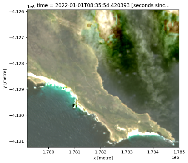
Dans l’exemple ci-dessous, nous allons charger des données de Landsat 9 du Cap pour l’Afrique du Sud en janvier 2022. Nous allons charger des données de trois bandes spectrales de satellites, ainsi que des données de masquage des nuages ('qa_aerosol'). En spécifiant output_crs='EPSG:6933' et resolution=(-30, 30), nous demandons à datacube de reprojeter nos données sur le système de référence de coordonnées africain Albers (CRS), avec des pixels de 30 x 30 m. Enfin, group_by='solar_day' garantit que les images superposées prises à quelques secondes d’intervalle lors du passage du satellite sont combinées en un seul pas de temps dans les données.
Remarque : pour une discussion plus générale sur la manière de charger des données à l’aide du datacube, reportez-vous au bloc-notes « Introduction au chargement des données <../Beginners_guide/03_Loading_data.ipynb> ».
[5]:
# load data
ds = dc.load(product="ls9_sr",
             measurements=['red', 'green', 'blue',
                           'qa_aerosol'],
             output_crs='EPSG:6933',
             y=(-34.31, -34.36),
             x=(18.44, 18.50),
             time=("2022-01", "2022-01"),
             resolution=(-30, 30),
             group_by="solar_day",
             )

print(ds)
<xarray.Dataset>
Dimensions:      (time: 2, y: 177, x: 194)
Coordinates:
  * time         (time) datetime64[ns] 2022-01-01T08:35:54.420393 2022-01-17T...
  * y            (y) float64 -4.126e+06 -4.126e+06 ... -4.131e+06 -4.131e+06
  * x            (x) float64 1.779e+06 1.779e+06 ... 1.785e+06 1.785e+06
    spatial_ref  int32 6933
Data variables:
    red          (time, y, x) uint16 8995 8851 8763 8678 ... 7172 7172 7163 7127
    green        (time, y, x) uint16 9122 8918 8850 8762 ... 7584 7584 7578 7518
    blue         (time, y, x) uint16 8176 8071 8021 7965 ... 7531 7531 7545 7516
    qa_aerosol   (time, y, x) uint8 160 160 160 160 160 ... 164 164 164 164 164
Attributes:
    crs:           EPSG:6933
    grid_mapping:  spatial_ref
Tracé des données Landsat
Nous pouvons tracer les données que nous avons chargées à l’aide de la fonction « rgb ». Par défaut, la fonction tracera les données sous forme d’image en vraies couleurs à l’aide des bandes « rouge », « verte » et « bleue ».
[6]:
rgb(ds, index=0)
Charger Landsat en utilisant load_ard
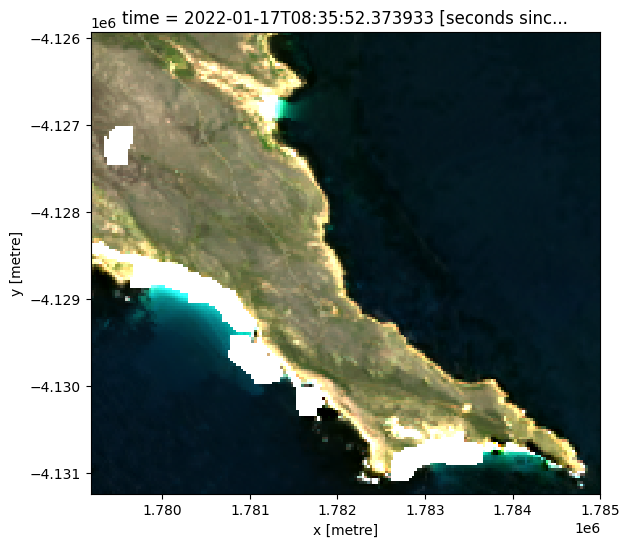
load_ard applique la mise à l’échelle linéaire et le décalage qui convertissent les données natives uint16 en valeurs réelles de réflectance de surface. load_ard concaténera et triera en outre les observations par heure et appliquera un masque de nuage. Le résultat est un ensemble de données prêt à être analysé.
Dans l’exemple ci-dessous, nous chargeons les données Landsat 9 pour la même heure et le même endroit que ci-dessus. Notez qu’un masque de nuages a maintenant été appliqué et que les données ont été converties en valeurs décimales de réflectance de surface.
Cette fonction chargera également les images de tous les capteurs Landsat s’ils sont ajoutés à l’argument « produits » sous forme de liste.
Vous pouvez trouver plus d’informations sur cette fonction dans le bloc-notes Using load ard.
[7]:
ds = load_ard(dc=dc,
              products=["ls9_sr"],
              measurements=['red', 'green', 'blue'],
              output_crs='EPSG:6933',
              y=(-34.31, -34.36),
              x=(18.44, 18.50),
              time=("2022-01", "2022-01"),
              resolution=(-30, 30),
              group_by="solar_day"
             )

print(ds)
Using pixel quality parameters for USGS Collection 2
Finding datasets
    ls9_sr
Applying pixel quality/cloud mask
Re-scaling Landsat C2 data
Loading 1 time steps
<xarray.Dataset>
Dimensions:      (time: 1, y: 177, x: 194)
Coordinates:
  * time         (time) datetime64[ns] 2022-01-17T08:35:52.373933
  * y            (y) float64 -4.126e+06 -4.126e+06 ... -4.131e+06 -4.131e+06
  * x            (x) float64 1.779e+06 1.779e+06 ... 1.785e+06 1.785e+06
    spatial_ref  int32 6933
Data variables:
    red          (time, y, x) float32 0.04758 0.04527 ... -0.003018 -0.004008
    green        (time, y, x) float32 0.04888 0.04618 ... 0.008395 0.006745
    blue         (time, y, x) float32 0.03158 0.02806 ... 0.007488 0.00669
Attributes:
    crs:           EPSG:6933
    grid_mapping:  spatial_ref
/usr/local/lib/python3.10/dist-packages/rasterio/warp.py:344: NotGeoreferencedWarning: Dataset has no geotransform, gcps, or rpcs. The identity matrix will be returned.
  _reproject(
Tracez les données Landsat masquées par les nuages :
[8]:
rgb(ds, index=0)
Informations Complémentaires
Licence : Le code de ce carnet est sous licence Apache, version 2.0 <https://www.apache.org/licenses/LICENSE-2.0>. Les données de Digital Earth Africa sont sous licence Creative Commons par attribution 4.0 <https://creativecommons.org/licenses/by/4.0/>.
Contact : Si vous avez besoin d’aide, veuillez poster une question sur le canal Slack Open Data Cube <http://slack.opendatacube.org/>`__ ou sur le GIS Stack Exchange en utilisant la balise open-data-cube (vous pouvez consulter les questions posées précédemment ici). Si vous souhaitez signaler un problème avec ce bloc-notes, vous pouvez en déposer un sur Github.
Version de Datacube compatible :
[9]:
print(datacube.__version__)
1.8.15
Dernier test :
[10]:
from datetime import datetime
datetime.today().strftime('%Y-%m-%d')
[10]:
'2023-08-11'