Sentinel-1

• Produits utilisés : s1_rtc

Mots-clés données utilisées ; sentinel-1,:index:ensembles de données ; sentinel-1, index:SAR

Aperçu

La mission Sentinel-1 <https://sentinel.esa.int/web/sentinel/missions/sentinel-1>__ est composée d’une constellation de deux satellites radar à synthèse d’ouverture (SAR), Sentinel-1A et Sentinel-1B, partageant le même plan orbital. Sentinel-1 offre une capacité de double polarisation, des temps de revisite très courts et une livraison rapide des produits. La mission collecte actuellement des données tous les 12 jours au-dessus de l’Afrique à une résolution spatiale d’environ 20 m. Sentinel-1A a été lancé le 3 avril 2014 et Sentinel-1B a suivi le 25 avril 2016. Deux autres engins spatiaux (Sentinel-1C et Sentinel-1D) sont prévus pour remplacer les deux premiers satellites à la fin de leur durée de vie opérationnelle. Pour plus d’informations sur les plateformes et applications Sentinel-1, consultez le site Web de l’Agence spatiale européenne <https://www.esa.int/Applications/Observing_the_Earth/Copernicus/Sentinel-1>`__.

Les données SAR ont l’avantage de fonctionner à des longueurs d’onde non gênées par la couverture nuageuse et peuvent acquérir des données sur un site de jour comme de nuit. La mission Sentinel-1 est l’observatoire radar européen de l’initiative conjointe Copernicus de la Commission européenne (CE) et de l’Agence spatiale européenne (ESA) qui peut offrir une surveillance fiable et répétée de vastes zones avec son instrument SAR.

La rétrodiffusion radar mesure la quantité de rayonnement micro-onde réfléchie vers le centre depuis la surface du sol. Cette mesure est sensible à la rugosité de la surface, à la teneur en humidité et à la géométrie de visualisation. DEAfrica fournit la rétrodiffusion Sentinel-1 sous forme de gamma-0 (γ0) corrigé en fonction du terrain radiométrique (RTC) où la variation due aux changements de géométrie d’observation a été atténuée.

DE Africa fournit des données Sentinel-1 acquises en mode interférométrique à large bande (IW) et avec une double polarisation (VV et VH). La série temporelle de rétrodiffusion à double polarisation peut être utilisée dans des applications pour les forêts, l’agriculture, les zones humides et la classification de la couverture terrestre. La capacité du SAR à voir à travers les nuages le rend essentiel pour la cartographie et la surveillance des changements de couverture terrestre dans les zones tropicales humides.

La rétrodiffusion du DEAfrica Sentinel-1 est traitée pour être conforme à la spécification « CEOS Analysis Ready Data for Land (CARD4L) <https://ceos.org/ard/> ». Des informations techniques supplémentaires sont disponibles dans le « Guide de l’utilisateur DE Africa <https://docs.digitalearthafrica.org/en/latest/data_specs/Sentinel-1_specs.html> ».

Description

Dans ce notebook, nous allons charger les données de rétrodiffusion SAR corrigées du terrain radiométrique (RTC) de Sentinel-1.

Les sujets abordés comprennent :

1. Inspection du produit Sentinel-1 et des mesures disponibles dans le datacube

2. Utilisation de la fonction native « dc.load() » pour charger les données Sentinel-1

3. Utilisation de la fonction wrapper « load_ard » pour charger les données Sentinel-1 masquées

---

Commencer

Pour exécuter cette analyse, exécutez toutes les cellules du bloc-notes, en commençant par la cellule « Charger les packages ».

Charger des paquets

%matplotlib inline
import datacube
import sys
import math
import numpy as np
import matplotlib.pyplot as plt
from deafrica_tools.plotting import rgb
from deafrica_tools.plotting import display_map
from deafrica_tools.datahandling import load_ard

Se connecter au datacube

dc = datacube.Datacube(app="Sentinel_1")

Produits et mesures disponibles

Liste des produits

Nous pouvons utiliser la fonctionnalité « list_products » de Datacube pour inspecter les produits SAR de DE Africa disponibles dans le Datacube. Le tableau ci-dessous indique les noms des produits que nous utiliserons pour charger les données, une brève description des données et l’instrument satellite qui a acquis les données.

dc.list_products().loc[dc.list_products()['description'].str.contains('radar')]

	name	description	license	default_crs	default_resolution
name
s1_rtc	s1_rtc	Sentinel 1 Gamma0 normalised radar backscatter	CC-BY-4.0	None	None

product = "s1_rtc"

Liste des mesures

Nous pouvons examiner plus en détail les données disponibles pour chaque produit SAR à l’aide de la fonctionnalité « list_measurements » de Datacube. Le tableau ci-dessous répertorie chacune des mesures disponibles dans les données.

measurements = dc.list_measurements()
measurements.loc[product]

	name	dtype	units	nodata	aliases	flags_definition
measurement
vv	vv	float32	1	NaN	[VV]	NaN
vh	vh	float32	1	NaN	[VH]	NaN
angle	angle	uint8	1	255.0	[ANGLE, local_incidence_angle]	NaN
area	area	float32	1	NaN	[AREA, normalised_scattering_area]	NaN
mask	mask	uint8	1	0.0	[MASK]	{'qa': {'bits': [0, 1, 2, 3, 4, 5, 6, 7], 'val...

Le produit Sentinel-1 dispose de cinq mesures :

• Rétrodiffusion en deux polarisations, « VV » et « VH ». Les deux lettres correspondent aux polarisations de la lumière envoyée et reçue par le satellite. VV fait référence au satellite qui envoie de la lumière polarisée verticalement et reçoit en retour de la lumière polarisée verticalement, tandis que VH fait référence au satellite qui envoie de la lumière polarisée verticalement et reçoit en retour de la lumière polarisée horizontalement.

• Un masque de données, avec « 0 » pour « aucune donnée », « 1 » pour des données valides et « 2 » pour l’ombre radar dans/à proximité.

• Zone de diffusion, normalisation qui a été calculée à l’aide d’un modèle numérique d’élévation et appliquée pour obtenir une correction radiométrique du terrain.

• Angle d’incidence local.

Charger le jeu de données Sentinel-1 à l’aide de dc.load()

Maintenant que nous savons quels produits et mesures sont disponibles pour le produit, nous pouvons charger des données à partir du datacube en utilisant « dc.load ».

Dans l’exemple ci-dessous, nous chargerons Sentinel-1 pour une partie du Ghana en 2020.

Nous allons charger les données de deux bandes de polarisation, « VV » et « VH », ainsi que le masque de données (« mask »). Les données sont chargées dans le système de référence de coordonnées (CRS) EPSG:4326 natif. Elles peuvent être reprojetées si « output_crs » et « resolution » sont définis dans la requête.

Remarque : pour une discussion plus générale sur la manière de charger des données à l’aide du datacube, reportez-vous au bloc-notes « Introduction au chargement des données <../Beginners_guide/03_Loading_data.ipynb> ».

# Define the area of interest
latitude = 5.423
longitude = -0.464
buffer = 0.02
time = ('2020-12')

bands = ['vv','vh','mask']

Nous définirons également une direction d’orbite pour cette requête. Les données Sentinel-1 sont acquises soit en passes « ascendantes », soit en passes « descendantes ». Comme l’antenne est orientée vers la droite, les données acquises dans différentes directions d’orbite auront des géométries de visualisation différentes. Cela peut entraîner une différence dans les valeurs de rétrodiffusion, par exemple sur des zones nues ou à végétation clairsemée.

La majeure partie du continent africain est couverte régulièrement par des pass « ascendants ». Pour certains endroits, des pass « descendants » sont également disponibles.

Pour certaines applications, un utilisateur peut souhaiter utiliser des données provenant des deux sens. Dans ce cas, tout biais potentiel doit être évalué en premier.

orbit_direction = 'ascending'

#add spatio-temporal extent to the query
query = {
    'x': (longitude-buffer, longitude+buffer),
    'y': (latitude+buffer, latitude-buffer),
    'time':time,
    'sat_orbit_state': orbit_direction,
}

Visualiser la zone sélectionnée

display_map(x=(longitude-buffer, longitude+buffer), y=(latitude+buffer, latitude-buffer))

Make this Notebook Trusted to load map: File -> Trust Notebook

# loading the data with the mask band included
ds_S1 = dc.load(product='s1_rtc',
                measurements=bands,
                group_by="solar_day",
                **query)

print(ds_S1)

<xarray.Dataset>
Dimensions:      (time: 5, latitude: 200, longitude: 200)
Coordinates:
  * time         (time) datetime64[ns] 2020-12-06T18:18:24.900676 ... 2020-12...
  * latitude     (latitude) float64 5.443 5.443 5.443 ... 5.404 5.403 5.403
  * longitude    (longitude) float64 -0.4839 -0.4837 -0.4835 ... -0.4443 -0.4441
    spatial_ref  int32 4326
Data variables:
    vv           (time, latitude, longitude) float32 0.07447 0.1258 ... 0.01145
    vh           (time, latitude, longitude) float32 0.01536 ... 0.0003317
    mask         (time, latitude, longitude) uint8 1 1 1 1 1 1 1 ... 1 1 1 1 1 1
Attributes:
    crs:           EPSG:4326
    grid_mapping:  spatial_ref

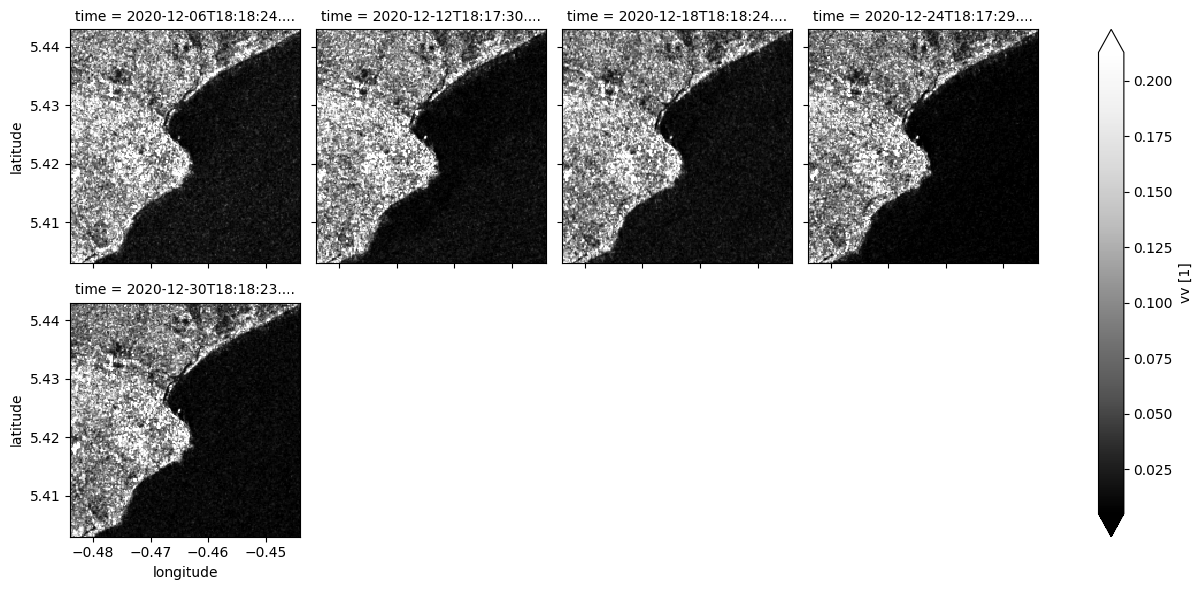
# Plot all VV observations for the year, and apply data mask to exclude pixels in and near radar shadow
ds_S1.vv.where(ds_S1.mask==1).plot(cmap="Greys_r", robust=True, col="time", col_wrap=4);

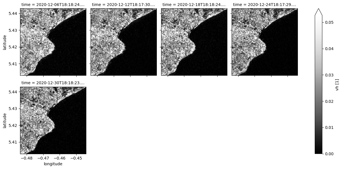
# Plot all VH observations for the year, and apply data mask to exclude pixels in and near radar shadow
ds_S1.vh.where(ds_S1.mask==1).plot(cmap="Greys_r", robust=True, col="time", col_wrap=4);

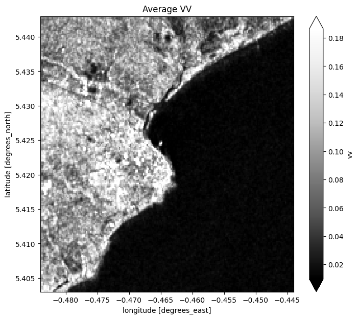
# Plot the average of all VV observations
mean_vv = ds_S1.vv.where(ds_S1.mask==1).mean(dim="time")

fig = plt.figure(figsize=(8, 7))
mean_vv.plot(cmap="Greys_r", robust=True)
plt.title("Average VV");

# Plot the average of all VH observations
mean_vh = ds_S1.vh.mean(dim="time")

fig = plt.figure(figsize=(8, 7))
mean_vh.plot(cmap="Greys_r", robust=True)
plt.title("Average VH");

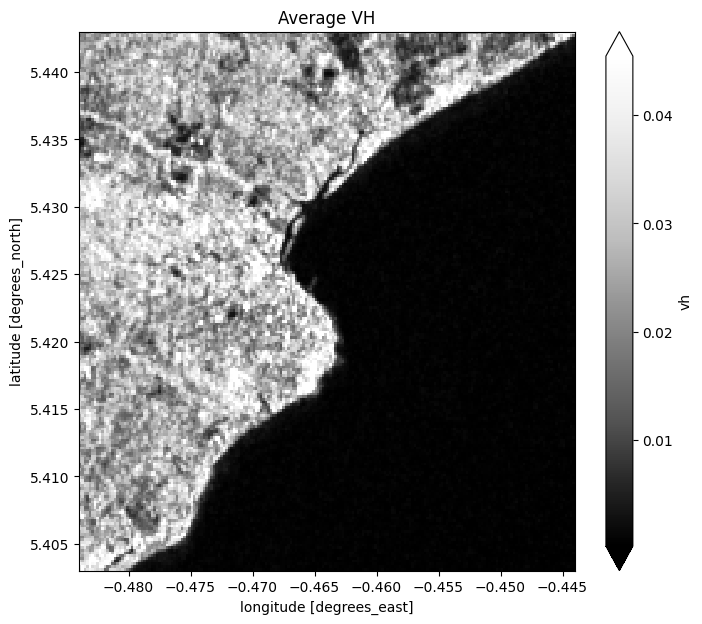
Une faible rétrodiffusion est mesurée au-dessus de l’eau en raison de la réflexion spéculaire.

Vous avez peut-être remarqué que l’eau dans les images individuelles VV et VH n’a pas une couleur uniforme. La distorsion que vous voyez est un type de bruit connu sous le nom de speckle, qui donne aux images un aspect granuleux. Le bruit de speckle peut être réduit grâce au filtrage. L’application d’un filtre speckle réduira le bruit et améliorera notre capacité à distinguer l’eau de la terre. Si vous êtes intéressé, vous pouvez trouver une introduction technique au filtrage speckle ici <https://web.archive.org/web/20200618064515/https://earth.esa.int/documents/653194/656796/Speckle_Filtering.pdf>.

#creation of a new band (VH/VV=vhvv) for RGB display
ds_S1['vhvv'] = ds_S1.vh.where(ds_S1.mask==1) / ds_S1.vv.where(ds_S1.mask==1)

# Set the timesteps to visualise
timesteps = [0,1,3]

# Generate RGB plots at each timestep
rgb(ds_S1.where(ds_S1.mask==1), bands=['vh','vv','vhvv'], index=timesteps)

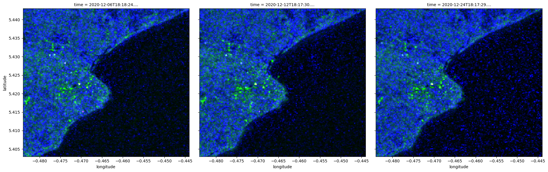
Dans les composites en fausses couleurs ci-dessus, une faible rétrodiffusion est mesurée au-dessus de l’eau qui apparaît noire ou bleu foncé. Une forte rétrodiffusion est mesurée dans les zones urbaines qui apparaissent vertes. Le sel et le poivre, également appelé bruit de mouchetures au-dessus de l’eau, sont également visibles.

Charger Sentinel-1 en utilisant load_ard

Cette fonction chargera les images de Sentinel-1 et appliquera un masque de qualité pixel. Le résultat est un ensemble de données prêt à être analysé, exempt d’ombres et de données manquantes.

Vous pouvez trouver plus d’informations sur cette fonction dans le bloc-notes Using load ard.

ds = load_ard(dc=dc,
              products=["s1_rtc"],
              measurements=['vv', 'vh'],
              group_by="solar_day",
              dtype='native',
              **query,
             )

print(ds)

Using pixel quality parameters for Sentinel 1
Finding datasets
    s1_rtc
Applying pixel quality/cloud mask
Loading 5 time steps
<xarray.Dataset>
Dimensions:      (time: 5, latitude: 200, longitude: 200)
Coordinates:
  * time         (time) datetime64[ns] 2020-12-06T18:18:24.900676 ... 2020-12...
  * latitude     (latitude) float64 5.443 5.443 5.443 ... 5.404 5.403 5.403
  * longitude    (longitude) float64 -0.4839 -0.4837 -0.4835 ... -0.4443 -0.4441
    spatial_ref  int32 4326
Data variables:
    vv           (time, latitude, longitude) float32 0.07447 0.1258 ... 0.01145
    vh           (time, latitude, longitude) float32 0.01536 ... 0.0003317
Attributes:
    crs:           EPSG:4326
    grid_mapping:  spatial_ref

Ci-dessous, nous traçons les données masquées de Sentinel-1 avec une haute qualité.

# Plot all VV observations for the year in which pixels in and near radar shadow have been excluded
ds.vv.plot(cmap="Greys_r", robust=True, col="time", col_wrap=4);

Analyse d’histogramme pour l’ensemble de données Sentinel-1

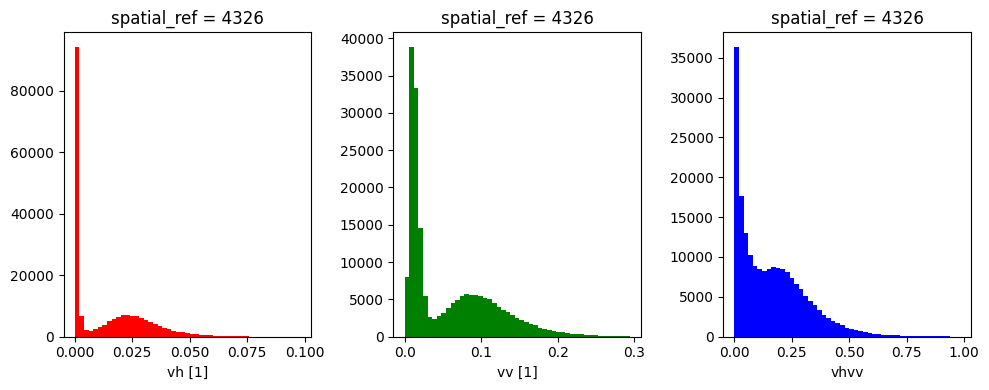
Les histogrammes ci-dessous montrent des distributions bimodales où une faible rétrodiffusion est mesurée sur l’eau.

#plotting each polorisation bands following converting to dB values
fig, ax = plt.subplots(1, 3, figsize=(10, 4))
ds_S1.vh.where(ds_S1.mask==1).plot.hist(ax=ax[0], bins=np.arange(0, 0.1, 0.002), facecolor='red')
ds_S1.vv.where(ds_S1.mask==1).plot.hist(ax=ax[1], bins=np.arange(0, 0.3, 0.006), facecolor='green')
ds_S1.vhvv.plot.hist(ax=ax[2], bins=np.arange(0, 1, 0.02), facecolor='blue')
plt.tight_layout()

---

Informations Complémentaires

Licence : Le code de ce carnet est sous licence Apache, version 2.0 <https://www.apache.org/licenses/LICENSE-2.0>. Les données de Digital Earth Africa sont sous licence Creative Commons par attribution 4.0 <https://creativecommons.org/licenses/by/4.0/>.

Contact : Si vous avez besoin d’aide, veuillez poster une question sur le canal Slack Open Data Cube <http://slack.opendatacube.org/>`__ ou sur le GIS Stack Exchange en utilisant la balise open-data-cube (vous pouvez consulter les questions posées précédemment ici). Si vous souhaitez signaler un problème avec ce bloc-notes, vous pouvez en déposer un sur Github.

Version de Datacube compatible :

print(datacube.__version__)

1.8.15

Dernier test :

from datetime import datetime
datetime.today().strftime('%Y-%m-%d')

'2023-08-11'