Calcul des indices de bande avec le package Spyndex
Produits utilisés : s2_l2a
Mots-clés données utilisées ; sentinel-2, index de bande ; NDVI, package de bande ; load_ard, index de bande ; EVIpackage ; spyndex`
Aperçu
Les indices de télédétection sont des combinaisons de bandes spectrales utilisées pour mettre en évidence les caractéristiques des données et du paysage sous-jacent. Le package Python Spyndex <https://www.nature.com/articles/s41597-023-02096-0> permet d’accéder aux indices spectraux du catalogue Awesome Spectral Indices. Il s’agit d’une liste standardisée, prête à l’emploi et organisée d’indices spectraux. Le package Spyndex comprend actuellement 232 indices optiques et radar <https://github.com/awesome-spectral-indices/awesome-spectral-indices/blob/main/output/spectral-indices-table.csv>.
L’un des avantages de ce package est le grand nombre d’indices « optiques et radar » disponibles pour les utilisateurs du sandbox DE Africa afin de calculer facilement une large gamme d’indices de télédétection qui peuvent être utilisés pour aider à cartographier et à surveiller des caractéristiques telles que la végétation et l’eau de manière cohérente dans le temps, ou comme entrées pour les algorithmes d’apprentissage automatique ou de classification utilisant les archives de données satellite prêtes à être analysées de Digital Earth Africa.
Description
Ce cahier montre comment :
Charger les archives de données satellite prêtes à être analysées de Digital Earth Africa à l’aide de « load_ard »
Calculer une gamme d’indices de végétation à l’aide de la fonction « spyndex »
Tracer les résultats pour tous les indices
Commencer
Pour exécuter cette analyse, exécutez toutes les cellules du bloc-notes, en commençant par la cellule « Charger les packages ».
Charger des paquets
[1]:
# Load the python packages.
%matplotlib inline

import matplotlib.pyplot as plt
import geopandas as gpd

#import spyndex package
import spyndex

import datacube

from deafrica_tools.datahandling import load_ard, mostcommon_crs
from deafrica_tools.plotting import rgb
from deafrica_tools.bandindices import calculate_indices
from odc.geo.geom import Geometry
from deafrica_tools.areaofinterest import define_area
Se connecter au datacube
Connectez-vous à la base de données Datacube pour activer le chargement des données de Digital Earth Africa.
[2]:
# Connect to the datacube
dc = datacube.Datacube(app="spyndex_function")
Sélectionnez l’emplacement
En utilisant la fonction define_area, sélectionnez la zone d’intérêt en spécifiant lat, lon et buffer. Si vous avez le vecteur ou le fichier de formes, décommentez le code ci-dessous Méthode 2 et remplacez aoi.shp par le chemin de votre fichier de formes.
[3]:
# Method 1: Specify the latitude, longitude, and buffer
aoi = define_area(lat=31.23394, lon=31.05560, buffer=0.02)

# Method 2: Use a polygon as a GeoJSON or Esri Shapefile.
#aoi = define_area(vector_path='aoi.shp')

#Create a geopolygon and geodataframe of the area of interest
geopolygon = Geometry(aoi["features"][0]["geometry"], crs="epsg:4326")
geopolygon_gdf = gpd.GeoDataFrame(geometry=[geopolygon], crs=geopolygon.crs)

# Get the latitude and longitude range of the geopolygon
lat_range = (geopolygon_gdf.total_bounds[1], geopolygon_gdf.total_bounds[3])
lon_range = (geopolygon_gdf.total_bounds[0], geopolygon_gdf.total_bounds[2])
Créer une requête et charger des données satellite
Pour démontrer comment calculer un indice de télédétection, nous devons d’abord charger des séries chronologiques de données satellitaires pour une zone. Les données satellitaires Sentinel-2 seront utilisées :
Il est fortement recommandé de charger les données avec load_ard lors du calcul des indices. En effet, load_ard effectue le nettoyage et la mise à l’échelle des données nécessaires pour des résultats d’index plus robustes. Reportez-vous à Using_load_ard pour en savoir plus
[4]:
# time_range.
time_range = ("2019-06", "2020-06")


# Create a reusable query object.
query = {
    "x": lon_range,
    "y": lat_range,
    "time": time_range,
    "resolution": (-10, 10)
}

# Identify the most common projection system in the input query
output_crs = mostcommon_crs(dc=dc, product="s2_l2a", query=query)

# Load available data from Sentinel-2 and filter to retain only times
# with at least 99% good data
ds = load_ard(
    dc=dc,
    products=["s2_l2a"],
    min_gooddata=0.99,
    measurements=["red", "green", "blue", "nir"],
    output_crs=output_crs,
    **query
)
Using pixel quality parameters for Sentinel 2
Finding datasets
    s2_l2a
Counting good quality pixels for each time step
/opt/venv/lib/python3.12/site-packages/rasterio/warp.py:387: NotGeoreferencedWarning: Dataset has no geotransform, gcps, or rpcs. The identity matrix will be returned.
  dest = _reproject(
Filtering to 78 out of 158 time steps with at least 99.0% good quality pixels
Applying pixel quality/cloud mask
Loading 78 time steps
Sélection d’une diapositive temporelle
[5]:
ds = ds.isel(time=[4, 11, 15, 23])
#### Imprimer le jeu de données xarray
[6]:
print(ds)
<xarray.Dataset> Size: 11MB
Dimensions:      (time: 4, y: 451, x: 390)
Coordinates:
  * time         (time) datetime64[ns] 32B 2019-06-21T08:51:41 ... 2019-09-11...
  * y            (y) float64 4kB 3.459e+06 3.459e+06 ... 3.455e+06 3.455e+06
  * x            (x) float64 3kB 3.129e+05 3.129e+05 ... 3.167e+05 3.168e+05
    spatial_ref  int32 4B 32636
Data variables:
    red          (time, y, x) float32 3MB 530.0 527.0 538.0 ... nan nan nan
    green        (time, y, x) float32 3MB 550.0 533.0 526.0 ... nan nan nan
    blue         (time, y, x) float32 3MB 326.0 344.0 338.0 ... nan nan nan
    nir          (time, y, x) float32 3MB 1.142e+03 1.112e+03 ... nan nan
Attributes:
    crs:           epsg:32636
    grid_mapping:  spatial_ref
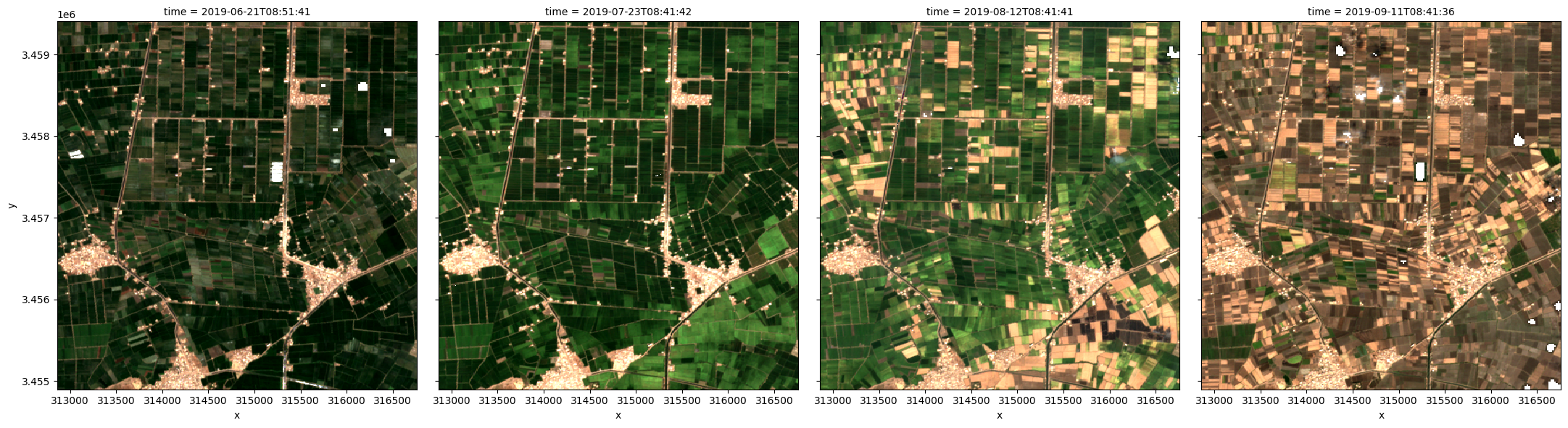
Tracez les images en vraies couleurs
La fonction « rgb » est utilisée pour tracer les pas de temps dans notre ensemble de données sous forme d’images RVB en couleurs réelles :
[7]:
rgb(ds, col='time')
Affichage des attributs d’un index
spyndex.indices[indexName] fournit les spécifications de l’indice d’intérêt. La cellule ci-dessous imprime les informations pour le NDVI
[8]:
print(spyndex.indices["NDVI"])
NDVI: Normalized Difference Vegetation Index
        * Application Domain: vegetation
        * Bands/Parameters: ['N', 'R']
        * Formula: (N-R)/(N+R)
        * Reference: https://ntrs.nasa.gov/citations/19740022614
Calculez l’indice de végétation par différence normalisée à l’aide de la méthode « spectral computeIndex ».
La cellule ci-dessous montre comment Singdex calcule les indices spectraux à l’aide de la fonction « spectral computeindex ». La fonction « spectral computeindex » prend la
argument « index » et il spécifie les indices spectraux à calculer
L’argument « params » prend les bandes de l’ensemble de données DE Africa et son nom de formule correspondant affiché dans « print(spyndex.indices[« NDVI »]) » ci-dessus. « NDVI » NDVI nécessite les bandes « N » et « R » en entrée qui sont définies pour l’ensemble de données DE Africa comme « ds.nir » et « ds.red ».
[9]:
ds["NDVI"] = spyndex.computeIndex(
    index=["NDVI"],
    params={
        "N": ds.nir,
        "R": ds.red
    }
)
Calculer l’indice de végétation amélioré à l’aide de Spyndex
L’utilisation de « spyndex.indices[indexName] » donne les détails de l’indice spectral utilisé. La cellule ci-dessous imprime des informations concernant l’indice spectral « EVI ».
[10]:
print(spyndex.indices["EVI"])
EVI: Enhanced Vegetation Index
        * Application Domain: vegetation
        * Bands/Parameters: ['g', 'N', 'R', 'C1', 'C2', 'B', 'L']
        * Formula: g*(N-R)/(N+C1*R-C2*B+L)
        * Reference: https://doi.org/10.1016/S0034-4257(96)00112-5
Calculez l’indice de végétation amélioré à l’aide de la méthode « spectral computeIndex ».
L”« EVI » a des valeurs constantes pour son calcul, comme nous pouvons le voir dans la formule ci-dessus.
Le package Spyndex fournit des valeurs constantes par défaut qui peuvent également être écrasées. Les constants sont accessibles à l’aide de spyndex.constants comme indiqué ci-dessous.
[11]:
ds["EVI"] = spyndex.computeIndex(
    index=["EVI"],
    params={
        "C1": spyndex.constants["C1"].value,
        "C2": spyndex.constants["C2"].value,
        "g": spyndex.constants["g"].value,
        "L": spyndex.constants["L"].value,
        "N": ds.nir,
        "R": ds.red,
        "B": ds.blue,
    },
)
Normalisation
La fonction « calculate_indices » de « deafrica_tools » normalise les valeurs Sentinel-2 selon une valeur de réflectance de surface maximale de « 10 000 ». Nous pouvons adapter le calcul Spyndex, comme ci-dessous, pour correspondre à cette procédure de normalisation.
[12]:
ds["EVI"] = spyndex.computeIndex(
    index=["EVI"],
    params={
        "C1": spyndex.constants["C1"].value,
        "C2": spyndex.constants["C2"].value,
        "g": spyndex.constants["g"].value,
        "L": spyndex.constants["L"].value,
        "N": ds.nir/10000,
        "R": ds.red/10000,
        "B": ds.blue/10000,
    },
)
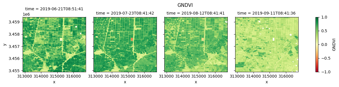
Indice de végétation par différence normalisée verte (GNDVI)
L’indice de végétation par différence normalisée verte GNDVI est un indice de végétation permettant d’estimer l’activité photosynthétique et est couramment utilisé pour déterminer l’absorption d’eau et d’azote par la canopée végétale. Le GNDVI est plus sensible à la variation de la chlorophylle dans la culture et a un point de saturation plus élevé que le NDVI. Il peut être utilisé dans les cultures à canopée dense ou à des stades de développement plus avancés. Vous trouverez plus d’informations dans la référence dans la cellule ci-dessous.
Affichage des attributs de l’indice de végétation normalisé par différence verte
[13]:
print(spyndex.indices["GNDVI"])
GNDVI: Green Normalized Difference Vegetation Index
        * Application Domain: vegetation
        * Bands/Parameters: ['N', 'G']
        * Formula: (N-G)/(N+G)
        * Reference: https://doi.org/10.1016/S0034-4257(96)00072-7
Calculer l’indice de végétation normalisé par différence verte à l’aide de Spyndex
[14]:
ds["GNDVI"] = spyndex.computeIndex(
    index=["GNDVI"],
    params={
        "N": ds.nir,
        "G": ds.green
    }
)
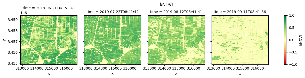
Indice de végétation à différence normalisée par noyau (kNDVI)
Le NDVI ne peut capturer que les relations linéaires entre la différence proche infrarouge (NIR) et le rouge et un paramètre d’intérêt, comme la biomasse verte. En réalité, cette relation est non linéaire. Le NDVI à noyau (kNDVI) a été développé <https://www.science.org/doi/10.1126/sciadv.abc7447>`__ pour tenir compte des relations d’ordre supérieur entre les canaux spectraux avec une généralisation non linéaire de l’indice de végétation par différence normalisée (NDVI) couramment utilisé. Il a été démontré que le kNDVI produit des estimations plus précises de variables physiques clés telles que la productivité primaire brute.
[15]:
print(spyndex.indices["kNDVI"])
kNDVI: Kernel Normalized Difference Vegetation Index
        * Application Domain: kernel
        * Bands/Parameters: ['kNN', 'kNR']
        * Formula: (kNN-kNR)/(kNN+kNR)
        * Reference: https://doi.org/10.1126/sciadv.abc7447
[16]:
# Use the computeKernel() method to compute the required kernel for kernel indices like the kNDVI
# Kernel Normalized Difference Vegetation Index
parameters = {
    "kNN": 1.0,
    "kNR": spyndex.computeKernel(
        kernel="RBF",
        params={"a": ds.nir , "b": ds.red, "sigma": 0.5 * (ds.nir + ds.red)},
    ),
}
ds["kNDVI"] = spyndex.computeIndex("kNDVI", parameters)
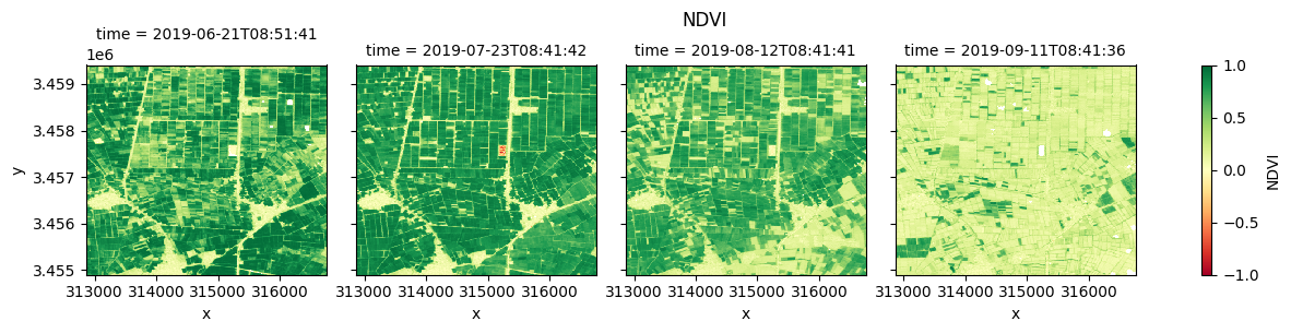
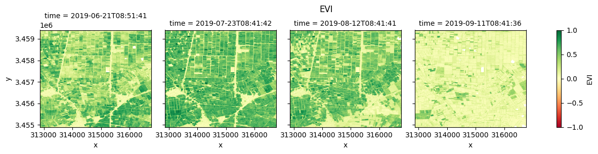
Tracer chaque indice de végétation
Le graphique ci-dessous permet de comparer les indices NDVI, EVI, GNDVI et kNDVI. Observez-vous des différences entre les indices ? Par exemple, il semble y avoir plus de saturation (plus grande fréquence de valeurs plus élevées/plus vertes) pour le NDVI et le GNDVI au cours du pas de temps de juillet par rapport à l’EVI et au kNDVI.
[17]:
#NDVI
fig_ndvi = ds.NDVI.clip(-1,1).plot(col="time", cmap="RdYlGn", vmin=-1, vmax=1)
fig_ndvi.fig.suptitle("NDVI", y= 1.0)
#EVI
fig_evi = ds.EVI.clip(-1,1).plot(col="time", cmap="RdYlGn", vmin=-1, vmax=1)
fig_evi.fig.suptitle("EVI", y= 1.0);
#GNDVI
fig_gndvi = ds.GNDVI.clip(-1,1).plot(col="time", cmap="RdYlGn", vmin=-1, vmax=1)
fig_gndvi.fig.suptitle("GNDVI", y= 1.0)
#kNDVI
fig_kndvi = ds.kNDVI.clip(-1,1).plot(col="time", cmap="RdYlGn", vmin=-1, vmax=1)
fig_kndvi.fig.suptitle("kNDVI", y= 1.0)
plt.show()
Conclusion
Ce bloc-notes montre comment le « paquet Spyndex » peut être utilisé avec les ensembles de données DE Africa pour calculer les indices spectraux. Il existe 232 indices optiques et radar <https://github.com/awesome-spectral-indices/awesome-spectral-indices/blob/main/output/spectral-indices-table.csv> » disponibles via le paquet, essayez-le et modifiez le bloc-notes pour tester différents indices et leurs résultats.
Informations Complémentaires
Licence : Le code de ce carnet est sous licence Apache, version 2.0 <https://www.apache.org/licenses/LICENSE-2.0>. Les données de Digital Earth Africa sont sous licence Creative Commons par attribution 4.0 <https://creativecommons.org/licenses/by/4.0/>.
Contact : Si vous avez besoin d’aide, veuillez poster une question sur le canal Slack Open Data Cube <http://slack.opendatacube.org/>`__ ou sur le GIS Stack Exchange en utilisant la balise open-data-cube (vous pouvez consulter les questions posées précédemment ici). Si vous souhaitez signaler un problème avec ce bloc-notes, vous pouvez en déposer un sur Github.
Version de Datacube compatible :
[18]:
print(datacube.__version__)
1.8.20
Dernier test :
[19]:
from datetime import date
print(date.today())
2025-01-15