Travailler avec le temps dans xarray
Produits utilisés : s2_l2a
Mots clés analyse; séries chronologiques, données utilisées; sentinel-2, méthodes de données; groupby,:index:méthodes de données; le plus proche, index:méthodes de données; interpolation, méthodes de données; rééchantillonnage, méthodes de données; composition
Aperçu
Les données de séries chronologiques <https://en.wikipedia.org/wiki/Time_series> sont une série de points de données généralement capturés à des moments successifs dans le temps. Dans un contexte de télédétection, les données de séries chronologiques sont une séquence d’images satellite discrètes prises dans la même zone à des moments successifs. L’analyse des séries chronologiques utilise différentes méthodes pour extraire des statistiques, des modèles et d’autres caractéristiques significatives des données. Les données et l’analyse des séries chronologiques ont de nombreuses applications allant de la surveillance des cultures agricoles à la détection des changements naturels de la végétation, en passant par la cartographie de la prospectivité minérale et la modélisation de la hauteur des marées.
Description
Le package Python « xarray » fournit de nombreuses techniques utiles pour traiter les données de séries chronologiques qui peuvent être appliquées aux données de Digital Earth Africa. Ce bloc-notes montre comment utiliser les techniques « xarray » pour :
Sélectionnez différentes périodes de données (par exemple, année, mois, jour) à partir d’un « xarray.Dataset »
Utiliser les accesseurs datetime pour extraire des informations supplémentaires de la dimension « temps » d’un ensemble de données
Résumer les données de séries chronologiques pour différentes périodes à l’aide de « .groupby() » et « .resample() »
Interpoler des données de séries chronologiques pour estimer les conditions du paysage à une date précise que le satellite n’a pas observées
Pour plus d’informations sur les techniques présentées ci-dessous, reportez-vous au guide des données de séries chronologiques « xarray » <http://xarray.pydata.org/en/stable/time-series.html>`__.
Commencer
Pour exécuter cette analyse, exécutez toutes les cellules du bloc-notes, en commençant par la cellule « Charger les packages ».
Charger des paquets
[1]:
%matplotlib inline

import datacube
import matplotlib.pyplot as plt
import numpy as np
import geopandas as gpd
from odc.geo.geom import Geometry

from deafrica_tools.datahandling import load_ard, mostcommon_crs
from deafrica_tools.areaofinterest import define_area
Se connecter au datacube
[2]:
dc = datacube.Datacube(app='Working_with_time')
Chargement des données Landsat
Tout d’abord, nous chargeons environ deux ans de données Sentinel-2, en utilisant la fonction load_ard et en filtrant les pas de temps avec au moins 95 % de pixels de bonne qualité.
Pour définir la zone d’intérêt, deux méthodes sont disponibles :
En spécifiant la latitude, la longitude et la zone tampon. Cette méthode nécessite que vous saisissiez la latitude centrale, la longitude centrale et la valeur de la zone tampon en degrés carrés autour du point central que vous souhaitez analyser. Par exemple, « lat = 10,338 », « lon = -1,055 » et « buffer = 0,1 » sélectionneront une zone avec un rayon de 0,1 degré carré autour du point avec les coordonnées (10,338, -1,055).
By uploading a polygon as a
GeoJSON or Esri Shapefile. If you choose this option, you will need to upload the geojson or ESRI shapefile into the Sandbox using Upload Files button in the top left corner of the Jupyter Notebook interface. ESRI shapefiles must be uploaded with all the related files
 (.cpg, .dbf, .shp, .shx). Once uploaded, you can use the shapefile or geojson to define the area of interest. Remember to update the code to call the file you have uploaded.
Pour utiliser l’une de ces méthodes, vous pouvez décommenter la ligne de code concernée et commenter l’autre. Pour commenter une ligne, ajoutez le symbole "#" avant le code que vous souhaitez commenter. Par défaut, la première option qui définit l’emplacement à l’aide de la latitude, de la longitude et du tampon est utilisée.
[3]:
# Define the location
# Method 1: Specify the latitude, longitude, and buffer
aoi = define_area(lat=13.94, lon=-16.54, buffer=0.125)

# Method 2: Use a polygon as a GeoJSON or Esri Shapefile.
# aoi = define_area(vector_path='aoi.shp')

#Create a geopolygon and geodataframe of the area of interest
geopolygon = Geometry(aoi["features"][0]["geometry"], crs="epsg:4326")
geopolygon_gdf = gpd.GeoDataFrame(geometry=[geopolygon], crs=geopolygon.crs)

# Get the latitude and longitude range of the geopolygon
lat_range = (geopolygon_gdf.total_bounds[1], geopolygon_gdf.total_bounds[3])
lon_range = (geopolygon_gdf.total_bounds[0], geopolygon_gdf.total_bounds[2])


# Create a reusable query
query = {
    'x': lon_range,
    'y': lat_range,
    'time': ('2018-01', '2019-12'),
    'resolution': (-20, 20),
    'measurements':['red', 'green', 'blue', 'nir']
}

# Identify the most common projection system in the input query
output_crs = mostcommon_crs(dc=dc, product='s2_l2a', query=query)

# Load available data from Landsat 8 and filter to retain only times
# with at least 95% good data
ds = load_ard(dc=dc,
              products=['s2_l2a'],
              min_gooddata=0.95,
              output_crs=output_crs,
              align=(15, 15),
              **query)
Using pixel quality parameters for Sentinel 2
Finding datasets
    s2_l2a
Counting good quality pixels for each time step
Filtering to 43 out of 172 time steps with at least 95.0% good quality pixels
Applying pixel quality/cloud mask
Loading 43 time steps
Explorer les données de matrice X en utilisant le temps
Nous allons ici explorer plusieurs façons d’utiliser la dimension temporelle dans un « xarray.Dataset ». Cette section décrit la sélection, la synthèse et l’interpolation des données à des moments précis.
Indexation par heure
Nous pouvons sélectionner des données pour une année entière en passant une chaîne à .sel() :
[4]:
ds.sel(time='2018')
[4]:
<xarray.Dataset> Size: 455MB
Dimensions:      (time: 15, y: 1392, x: 1361)
Coordinates:
  * time         (time) datetime64[ns] 120B 2018-01-08T11:46:56 ... 2018-12-1...
  * y            (y) float64 11kB 1.556e+06 1.556e+06 ... 1.528e+06 1.528e+06
  * x            (x) float64 11kB 3.2e+05 3.2e+05 ... 3.472e+05 3.472e+05
    spatial_ref  int32 4B 32628
Data variables:
    red          (time, y, x) float32 114MB 2.254e+03 1.988e+03 ... 1.747e+03
    green        (time, y, x) float32 114MB 1.502e+03 1.348e+03 ... 1.336e+03
    blue         (time, y, x) float32 114MB 815.0 742.0 ... 1.016e+03 1.002e+03
    nir          (time, y, x) float32 114MB 3.789e+03 3.519e+03 ... 2.496e+03
Attributes:
    crs:           epsg:32628
grid_mapping: spatial_refOu sélectionnez un seul mois :
[5]:
ds.sel(time='2018-05')
[5]:
<xarray.Dataset> Size: 30MB
Dimensions:      (time: 1, y: 1392, x: 1361)
Coordinates:
  * time         (time) datetime64[ns] 8B 2018-05-23T11:39:00
  * y            (y) float64 11kB 1.556e+06 1.556e+06 ... 1.528e+06 1.528e+06
  * x            (x) float64 11kB 3.2e+05 3.2e+05 ... 3.472e+05 3.472e+05
    spatial_ref  int32 4B 32628
Data variables:
    red          (time, y, x) float32 8MB 2.626e+03 2.49e+03 ... 1.988e+03
    green        (time, y, x) float32 8MB 1.895e+03 1.793e+03 ... 1.542e+03
    blue         (time, y, x) float32 8MB 1.112e+03 1.08e+03 ... 1.132e+03
    nir          (time, y, x) float32 8MB 3.536e+03 3.472e+03 ... 2.686e+03
Attributes:
    crs:           epsg:32628
grid_mapping: spatial_refOu sélectionnez une plage de dates à l’aide de slice(). Cela sélectionne toutes les observations entre les deux dates, y compris les valeurs de début et de fin :
[6]:
ds.sel(time=slice('2018-06', '2019-01'))
[6]:
<xarray.Dataset> Size: 212MB
Dimensions:      (time: 7, y: 1392, x: 1361)
Coordinates:
  * time         (time) datetime64[ns] 56B 2018-07-22T11:47:38 ... 2019-01-18...
  * y            (y) float64 11kB 1.556e+06 1.556e+06 ... 1.528e+06 1.528e+06
  * x            (x) float64 11kB 3.2e+05 3.2e+05 ... 3.472e+05 3.472e+05
    spatial_ref  int32 4B 32628
Data variables:
    red          (time, y, x) float32 53MB 2.233e+03 2.212e+03 ... 1.951e+03
    green        (time, y, x) float32 53MB 1.566e+03 1.525e+03 ... 1.409e+03
    blue         (time, y, x) float32 53MB 486.0 557.0 ... 1.016e+03 976.0
    nir          (time, y, x) float32 53MB 3.711e+03 3.922e+03 ... 2.792e+03
Attributes:
    crs:           epsg:32628
grid_mapping: spatial_refPour sélectionner l’heure la plus proche d’une valeur de temps souhaitée, nous la définissons pour utiliser une méthode de voisin le plus proche, « nearest ». Nous devons spécifier l’heure à l’aide d’un objet « datetime », sinon l’indexation xarray suppose que nous sélectionnons une plage, comme l’exemple de mois « ds.sel(time=”2018-05”) » ci-dessus.
Ici, nous avons choisi une date au début de décembre 2018. « le plus proche » trouvera l’observation la plus proche de cette date.
[7]:
target_time = np.datetime64('2018-12-01')

ds.sel(time=target_time, method='nearest')
[7]:
<xarray.Dataset> Size: 30MB
Dimensions:      (y: 1392, x: 1361)
Coordinates:
    time         datetime64[ns] 8B 2018-12-09T11:47:28
  * y            (y) float64 11kB 1.556e+06 1.556e+06 ... 1.528e+06 1.528e+06
  * x            (x) float64 11kB 3.2e+05 3.2e+05 ... 3.472e+05 3.472e+05
    spatial_ref  int32 4B 32628
Data variables:
    red          (y, x) float32 8MB 2.376e+03 2.035e+03 ... 1.987e+03 1.938e+03
    green        (y, x) float32 8MB 1.61e+03 1.375e+03 ... 1.487e+03 1.416e+03
    blue         (y, x) float32 8MB 777.0 654.0 970.0 ... 1.051e+03 960.0
    nir          (y, x) float32 8MB 3.633e+03 3.515e+03 ... 2.866e+03 2.748e+03
Attributes:
    crs:           epsg:32628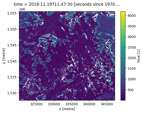
grid_mapping: spatial_refVous pouvez sélectionner l’heure la plus proche avant une heure donnée en utilisant « ffill » (remplissage vers l’avant).
[8]:
previous_time = ds.sel(time=target_time, method='ffill')

previous_time.blue.plot();
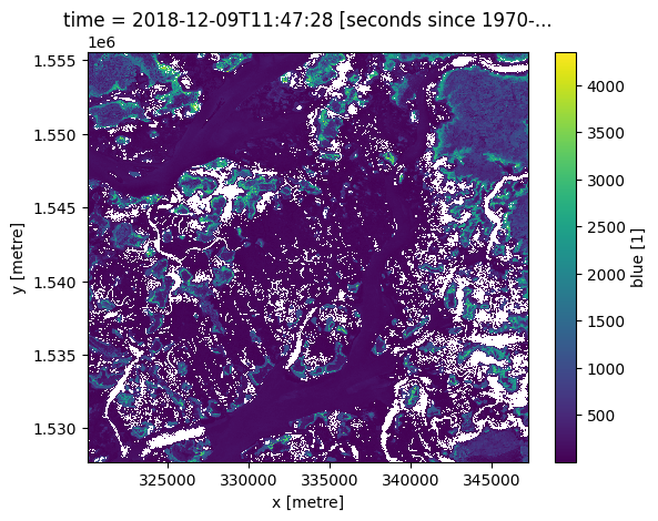
Pour sélectionner l’heure la plus proche après une heure donnée, utilisez « bfill » (back-fill).
[9]:
next_time = ds.sel(time=target_time, method='bfill')

next_time.blue.plot()
[9]:
<matplotlib.collections.QuadMesh at 0x7fe3691f6e10>
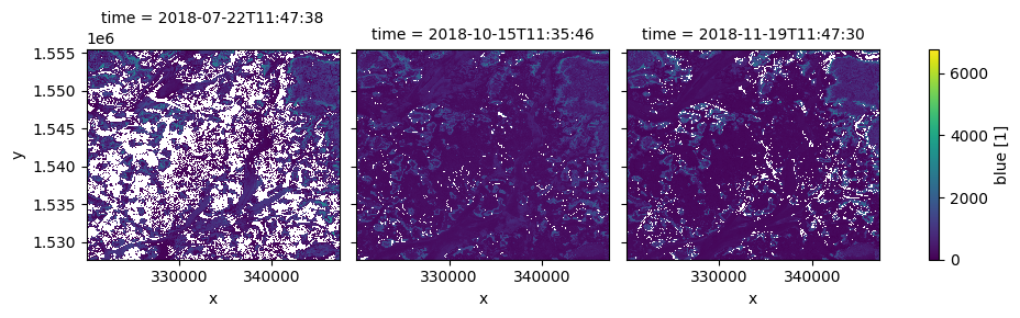
Les mêmes méthodes fonctionnent également sur une liste d’heures :
[10]:
many_times = np.array([
    '2018-06-23',
    '2018-09-13',
    '2018-11-02'
], dtype=np.datetime64)

nearest = ds.sel(time=many_times, method='nearest')

nearest.blue.plot(col='time', vmin=0);
Utilisation de l’accesseur datetime
« xarray » vous permet d’extraire facilement des informations supplémentaires de la dimension « temps » dans les données de Digital Earth Africa. Par exemple, nous pouvons obtenir une liste de la saison à laquelle appartient chaque observation :
[11]:
ds.time.dt.season
[11]:
<xarray.DataArray 'season' (time: 43)> Size: 516B
array(['DJF', 'DJF', 'DJF', 'DJF', 'DJF', 'MAM', 'MAM', 'MAM', 'MAM',
       'MAM', 'JJA', 'SON', 'SON', 'DJF', 'DJF', 'DJF', 'DJF', 'DJF',
       'DJF', 'MAM', 'MAM', 'MAM', 'MAM', 'MAM', 'MAM', 'MAM', 'MAM',
       'MAM', 'MAM', 'MAM', 'MAM', 'MAM', 'MAM', 'JJA', 'JJA', 'JJA',
       'SON', 'SON', 'SON', 'SON', 'SON', 'DJF', 'DJF'], dtype='<U3')
Coordinates:
  * time         (time) datetime64[ns] 344B 2018-01-08T11:46:56 ... 2019-12-2...
    spatial_ref  int32 4B 32628
Attributes:
units: seconds since 1970-01-01 00:00:00Ou le jour de l’année :
[12]:
ds.time.dt.dayofyear
[12]:
<xarray.DataArray 'dayofyear' (time: 43)> Size: 344B
array([  8,   8,  23,  48,  53,  63,  68,  73,  93, 143, 203, 288, 323,
       343, 348,   3,  18,  43,  53,  68,  73,  83,  83,  98,  98, 103,
       108, 108, 118, 123, 133, 143, 148, 158, 183, 188, 273, 293, 303,
       328, 333, 353, 358])
Coordinates:
  * time         (time) datetime64[ns] 344B 2018-01-08T11:46:56 ... 2019-12-2...
    spatial_ref  int32 4B 32628
Attributes: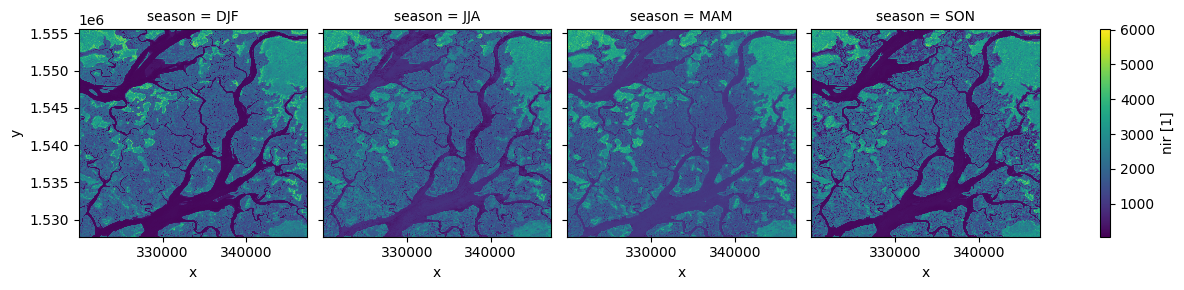
units: seconds since 1970-01-01 00:00:00Regroupement et rééchantillonnage par temps
« xarray » fournit également des raccourcis pour agréger des données au fil du temps. Dans l’exemple ci-dessous, nous regroupons d’abord nos données par saison, puis prenons la médiane de chaque groupe. Cela produit un nouvel ensemble de données avec seulement quatre observations (une par saison).
[13]:
# Group the time series into seasons, and take median of each time period
ds_seasonal = ds.groupby('time.season').median(dim='time')

# Plot the output
ds_seasonal.nir.plot(col='season', col_wrap=4)
plt.show()
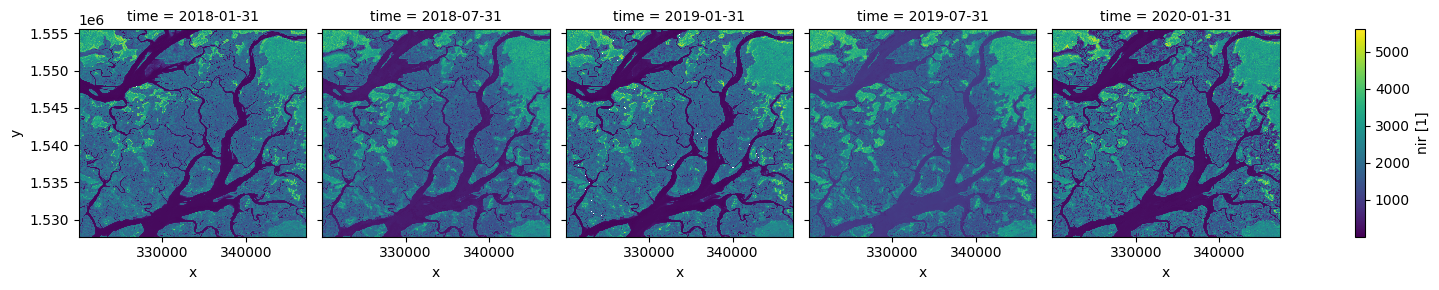
Nous pouvons également utiliser la méthode .resample() pour résumer notre ensemble de données en blocs de temps plus grands. Dans l’exemple ci-dessous, nous produisons une médiane composite pour chaque 6 mois de données dans notre ensemble de données :
[14]:
# Resample to combine each 6 months of data into a median composite
ds_resampled = ds.resample(time="6m").median()

# Plot the new resampled data
ds_resampled.nir.plot(col="time")
plt.show()
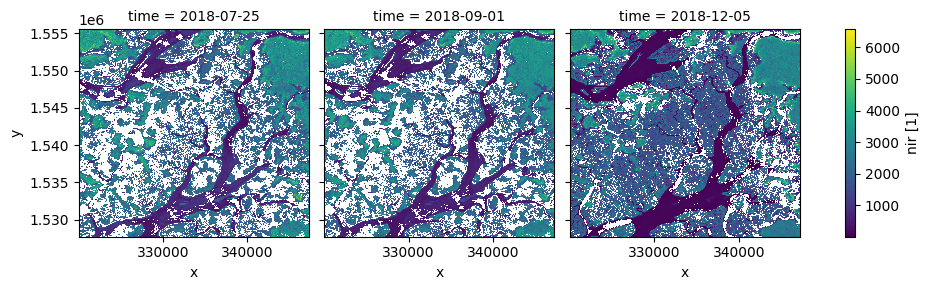
Interpolation de nouveaux pas de temps
Parfois, nous souhaitons obtenir des données pour des heures/dates spécifiques qui n’ont pas été observées par un satellite. Pour estimer à quoi ressemblait le paysage à certaines dates, nous pouvons utiliser la méthode .interp() pour interpoler entre les deux observations les plus proches.
Par défaut, la méthode interp() utilise une interpolation linéaire (method='linear'). Une autre option utile est method='nearest', qui renverra l’observation satellite la plus proche de la ou des dates spécifiées.
[15]:
# New dates to interpolate data for
new_dates = ['2018-07-25', '2018-09-01', '2018-12-05']

# Interpolate Landsat values for three new dates
ds_interp = ds.interp(time=new_dates)

# Plot the new interpolated data
ds_interp.nir.plot(col='time')
plt.show()
Informations Complémentaires
Licence:
Le code de ce bloc-notes est sous licence « Apache License, Version 2.0 <https://www.apache.org/licenses/LICENSE-2.0> ».
Les données de Digital Earth Africa sont sous licence Creative Commons Attribution 4.0 <https://creativecommons.org/licenses/by/4.0/>.
Contact:
Si vous avez besoin d’aide, veuillez poster une question sur le canal Slack Open Data Cube <http://slack.opendatacube.org/>`__ ou sur le GIS Stack Exchange en utilisant la balise open-data-cube (vous pouvez consulter les questions posées précédemment ici). Si vous souhaitez signaler un problème avec ce bloc-notes, vous pouvez en déposer un sur Github.
Version de Datacube compatible :
[16]:
print(datacube.__version__)
1.8.20
Dernier test :
[17]:
from datetime import datetime
datetime.today().strftime('%Y-%m-%d')
[17]:
'2025-01-15'