Application du masquage de bits WOfS

• Produits utilisés : wofs_ls

Mots clés données utilisées ; WOfS, méthodes de données ; wofs_fuser, analyse ; masquage

Aperçu

Le produit « Observations de l’eau depuis l’espace (WOfS) » <https://docs.digitalearthafrica.org/en/latest/data_specs/Landsat_WOfS_specs.html> montre l’eau observée par les satellites Landsat au-dessus de l’Afrique.

Les images individuelles classées selon l’eau sont appelées couches d’observation de l’eau (WOFL) et sont créées dans une relation 1 à 1 avec les données satellite d’entrée. Il existe donc une WOFL pour chaque ensemble de données satellite traité pour la présence d’eau.

Description

Ce cahier explique à la fois la structure des WOFL et comment vous pouvez l’utiliser pour un masquage d’image puissant et flexible.

Les données d’un WOFL sont stockées sous forme de champ binaire. Il s’agit d’un nombre binaire, où chaque chiffre du nombre est défini indépendamment ou non en fonction de la présence (1) ou de l’absence (0) d’un attribut particulier (eau, nuage, ombre de nuage, etc.). De cette manière, la valeur décimale unique associée à chaque pixel peut fournir des informations sur diverses caractéristiques de ce pixel.

Le cahier montre comment :

1. Charger les données WOFL pour un emplacement et une période donnés

2. Inspecter les informations du bit indicateur WOLF

3. Utilisez les indicateurs de bits WOFL pour créer un masque binaire

---

Commencer

Pour exécuter cette analyse, exécutez toutes les cellules du bloc-notes, en commençant par la cellule « Charger les packages ».

Une fois l’analyse terminée, vous pouvez modifier certaines valeurs dans la cellule « Paramètres d’analyse » et réexécuter l’analyse pour charger les WOFL pour un emplacement ou une période différente.

Charger des paquets

%matplotlib inline

import datacube
import numpy as np
import geopandas as gpd
import matplotlib.pyplot as plt
from datacube.utils import masking
from datacube.utils.geometry import Geometry

from deafrica_tools.plotting import display_map, plot_wofs
from deafrica_tools.datahandling import wofs_fuser, mostcommon_crs
from deafrica_tools.areaofinterest import define_area

Se connecter au datacube

dc = datacube.Datacube(app="Applying_WOfS_bitmasking")

Paramètres d’analyse

Pour charger les données WOFL, nous pouvons d’abord créer une requête réutilisable qui définira l’étendue spatiale et la période temporelle qui nous intéressent, ainsi que d’autres paramètres importants utilisés pour charger correctement les données.

Sélectionnez l’emplacement

Pour définir la zone d’intérêt, deux méthodes sont disponibles :

1. En spécifiant la latitude, la longitude et la zone tampon. Cette méthode nécessite que vous saisissiez la latitude centrale, la longitude centrale et la valeur de la zone tampon en degrés carrés autour du point central que vous souhaitez analyser. Par exemple, « lat = 10,338 », « lon = -1,055 » et « buffer = 0,1 » sélectionneront une zone avec un rayon de 0,1 degré carré autour du point avec les coordonnées (10,338, -1,055).

2. By uploading a polygon as a GeoJSON or Esri Shapefile. If you choose this option, you will need to upload the geojson or ESRI shapefile into the Sandbox using Upload Files button in the top left corner of the Jupyter Notebook interface. ESRI shapefiles must be uploaded with all the related files (.cpg, .dbf, .shp, .shx). Once uploaded, you can use the shapefile or geojson to define the area of interest. Remember to update the code to call the file you have uploaded.

Pour utiliser l’une de ces méthodes, vous pouvez décommenter la ligne de code concernée et commenter l’autre. Pour commenter une ligne, ajoutez le symbole "#" avant le code que vous souhaitez commenter. Par défaut, la première option qui définit l’emplacement à l’aide de la latitude, de la longitude et du tampon est utilisée.

Si vous exécutez le bloc-notes pour la première fois, conservez les paramètres par défaut ci-dessous. Cela permettra de démontrer le fonctionnement de l’analyse et de fournir des résultats significatifs.

# Method 1: Specify the latitude, longitude, and buffer
aoi = define_area(lat=-11.6216, lon=29.6987, buffer=0.175)

# Method 2: Use a polygon as a GeoJSON or Esri Shapefile.
# aoi = define_area(vector_path='aoi.shp')

#Create a geopolygon and geodataframe of the area of interest
geopolygon = Geometry(aoi["features"][0]["geometry"], crs="epsg:4326")
geopolygon_gdf = gpd.GeoDataFrame(geometry=[geopolygon], crs=geopolygon.crs)

# Get the latitude and longitude range of the geopolygon
lat_range = (geopolygon_gdf.total_bounds[1], geopolygon_gdf.total_bounds[3])
lon_range = (geopolygon_gdf.total_bounds[0], geopolygon_gdf.total_bounds[2])

# Create a reusable query
query = {
    'x': lon_range,
    'y': lat_range,
    'time': ('2018-10'),
    'resolution': (-30, 30)
}

Afficher l’emplacement sélectionné

display_map(x=lon_range,y=lat_range)

Make this Notebook Trusted to load map: File -> Trust Notebook

Charger les données WOFL

Les WOFL étant créés scène par scène et certaines scènes se chevauchant, il est important, lors du chargement des données dans « group_by » par jour solaire, de s’assurer que les données entre les scènes sont combinées correctement en utilisant la fonction WOfS « fuse_func ». Cela permettra de fusionner les observations prises le même jour et de garantir que les données importantes ne soient pas perdues lors de la combinaison des ensembles de données qui se chevauchent.

# Load the data from the datacube
output_crs = mostcommon_crs(dc=dc, product='wofs_ls', query=query)

wofls = dc.load(product="wofs_ls",
                output_crs=output_crs,
                group_by="solar_day",
                fuse_func=wofs_fuser,
                collection_category='T1', #only grab good georeferenced scenes
                **query)

/home/jovyan/dev/deafrica-sandbox-notebooks/Tools/deafrica_tools/datahandling.py:733: UserWarning: Multiple UTM zones ['epsg:32636', 'epsg:32635'] were returned for this query. Defaulting to the most common zone: epsg:32636
  warnings.warn(

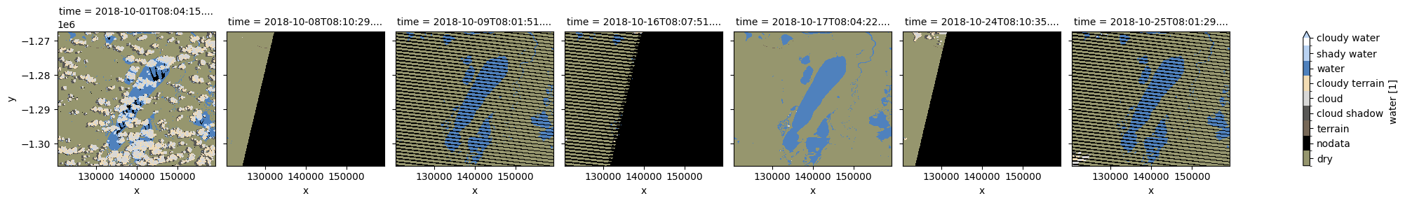
Tracez les WOFL chargés à l’aide de la fonction « plot_wofs »

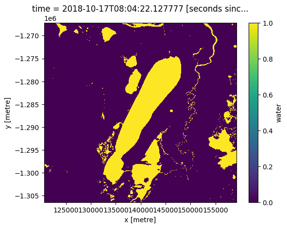
plot_wofs(wofls.water, col='time', col_wrap=7);

# Select one image of interest (`time=4` selects the fifth observation)
wofl = wofls.isel(time=4)

Comprendre les WOFL

Comme mentionné ci-dessus, les WOFL sont stockés sous forme de nombre binaire, où chaque chiffre du nombre est défini ou non de manière indépendante en fonction de la présence (1) ou de l’absence (0) d’une caractéristique particulière. Vous trouverez ci-dessous une répartition des bits représentant quelles caractéristiques, ainsi que la valeur décimale associée à ce bit défini sur true.

Attribut	Bit/position	Valeur décimale
Aucune donnée	0: 0------- ou 1-------	1
Non contigu	1: -0------ ou -1------	2
Mer (non utilisé)	2: --0----- ou --1-----	4
Terrain ou angle solaire faible	3: ---0---- ou ---1----	8
Pente élevée	4: ----0--- ou ----1---	16
Ombre de nuage	5: -----0-- ou -----1--	32
Nuage	6: ------0- ou ------1-	64
Eau	7: -------0 ou -------1	128

Les valeurs dans les tracés ci-dessus sont la représentation décimale de la combinaison des indicateurs définis. Par exemple, une valeur de 136 indique que de l’eau (128) ET une ombre du terrain / un angle solaire faible (8) ont été observés pour le pixel, tandis qu’une valeur de 144 indiquerait de l’eau (128) ET une pente élevée (16).

Ces informations sur le drapeau sont disponibles dans les données chargées et peuvent être visualisées comme ci-dessous

# Display details of available flags
flags = masking.describe_variable_flags(wofls)
flags["bits"] = flags["bits"].astype(str)
flags.sort_values(by="bits")

	bits	values	description
nodata	0	{'0': False, '1': True}	No data
noncontiguous	1	{'0': False, '1': True}	At least one EO band is missing or saturated
low_solar_angle	2	{'0': False, '1': True}	Low solar incidence angle
terrain_shadow	3	{'0': False, '1': True}	Terrain shadow
high_slope	4	{'0': False, '1': True}	High slope
cloud_shadow	5	{'0': False, '1': True}	Cloud shadow
cloud	6	{'0': False, '1': True}	Cloudy
water_observed	7	{'0': False, '1': True}	Classified as water by the decision tree
dry	[7, 6, 5, 4, 3, 2, 1, 0]	{'0': True}	No water detected
wet	[7, 6, 5, 4, 3, 2, 1, 0]	{'128': True}	Clear and Wet

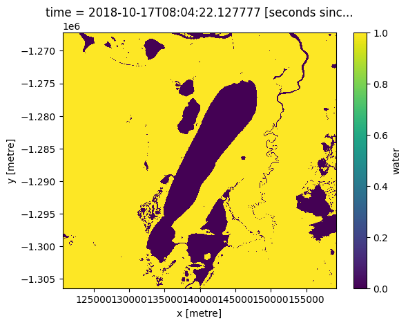
# Show areas flagged as water only (with no other flags set)
(wofl.water == 128).plot.imshow();

Masquage

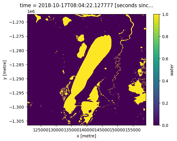
Nous pouvons convertir le champ de bits WOFL en un tableau binaire contenant les valeurs True et False. Cela nous permet d’utiliser les données WOFL comme un masque pouvant être appliqué à d’autres ensembles de données.

La fonction « make_mask » nous permet de créer un masque en utilisant les étiquettes d’indicateur (par exemple « humide » ou « sec ») plutôt que les nombres binaires que nous avons utilisés ci-dessus.

# Create a mask based on all 'wet' pixels
wetwofl = masking.make_mask(wofl, wet=True)
wetwofl.water.plot();

Créez des masques personnalisés en combinant des drapeaux

Les drapeaux peuvent être combinés. Lorsque des drapeaux sont enchaînés, ils sont combinés de manière logique. Ce processus fonctionne en transmettant un dictionnaire avec des valeurs vrai/faux à la fonction make_mask. Cela vous permet de choisir si vous souhaitez supprimer les nuages et/ou les ombres des nuages de l’imagerie.

# Clear (no clouds and shadow)
clear = {"cloud_shadow": False, "cloud": False}

cloudfree = masking.make_mask(wofl, **clear)
cloudfree.water.plot();

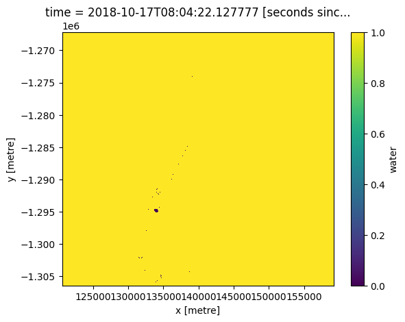
Ou, pour regarder uniquement les zones claires qui sont des données de bonne qualité et non humides, nous pouvons utiliser l’indicateur « sec ».

# clear and dry mask
good_data_mask = masking.make_mask(wofl, dry=True)
good_data_mask.water.plot();

---

Informations Complémentaires

Licence : Le code de ce carnet est sous licence Apache, version 2.0 <https://www.apache.org/licenses/LICENSE-2.0>. Les données de Digital Earth Africa sont sous licence Creative Commons par attribution 4.0 <https://creativecommons.org/licenses/by/4.0/>.

Contact : Si vous avez besoin d’aide, veuillez poster une question sur le canal Slack Open Data Cube <http://slack.opendatacube.org/>`__ ou sur le GIS Stack Exchange en utilisant la balise open-data-cube (vous pouvez consulter les questions posées précédemment ici). Si vous souhaitez signaler un problème avec ce bloc-notes, vous pouvez en déposer un sur Github.

Version de Datacube compatible :

print(datacube.__version__)

1.8.15

Dernier test :

from datetime import datetime
datetime.today().strftime('%Y-%m-%d')

'2023-08-11'