Génération de composites GeoMAD
Mots clés données utilisées ; sentinel-2, données utilisées ; landsat 8, index:données utilisées ; MAD, méthodes de données ; géomédiane, analyse ; composites, dask, méthodes de données ; rééchantillonnage, méthodes de données ; groupby
Aperçu
Les images individuelles de télédétection peuvent être affectées par des données bruyantes, notamment des nuages, des ombres de nuages et de la brume. Pour produire des images plus nettes qui peuvent être comparées plus facilement dans le temps, nous pouvons créer des images « récapitulatives » ou « composites » qui combinent plusieurs images en une seule image pour révéler l’apparence médiane ou « typique » du paysage pendant une certaine période.
Une approche consiste à créer un « géomédian » <https://github.com/daleroberts/hdmedians>. Un « géomédian » est basé sur une statistique de haute dimension appelée « médiane géométrique » (Small 1990) <https://www.jstor.org/stable/1403809), qui échange efficacement une pile temporelle d’observations de mauvaise qualité contre un seul composite de pixels de haute qualité avec un bruit spatial réduit (Roberts et al. 2017) <https://ieeexplore.ieee.org/abstract/document/8004469). Contrairement à une médiane standard, un géomédian maintient la relation entre les bandes spectrales. Cela nous permet d’effectuer des analyses plus approfondies sur les images composites comme nous le ferions sur les images satellites originales (par exemple en permettant le calcul d’indices de bande communs, comme le NDVI).
Le produit GEoMAD de DE Africa (Geomedian et Median Absolute Deviations), en plus de contenir les géomédianes des bandes de réflectance de surface, GeoMAD comprend également trois couches de déviation absolue médiane (MAD). Il s’agit de mesures statistiques d’ordre supérieur sur la variation par rapport à la géomédiane. Ces couches peuvent être utilisées seules ou avec la géomédiane pour obtenir des informations sur la surface terrestre et comprendre son évolution au fil du temps.
Toutes les données de la période sélectionnée doivent être chargées pour calculer un composite, de sorte que le calcul des géomédianes peut nécessiter beaucoup de calculs, en particulier sur de grandes zones ou de longues échelles de temps. Pour faciliter ces analyses, DE Africa héberge un certain nombre de produits geoMAD pré-calculés :
Sentinel-2 annuel GeoMAD de 2017 à aujourd’hui, avec le nom de produit
gm_s2_annualSentinel-2 semestriel (six mois) GeoMAD de 2019 à aujourd’hui, avec le nom de produit
gm_s2_semiannualGeoMAD annuel Landat de 2013 à aujourd’hui, avec le nom de produit
gm_ls8_annual
Cela réduit le temps et les ressources nécessaires pour calculer la géomédiane si vous effectuez une analyse sur une échelle de temps annuelle. Des instructions sur la façon d’utiliser la géomédiane de Sentinel-2 GeoMAD se trouvent dans le bloc-notes Datasets/GeoMAD.ipynb.
Pour les analyses sur d’autres échelles de temps, comme l’étude des changements au fil des saisons, il n’est pas possible d’utiliser le produit géomédian annuel. Dans ces cas, il peut être utile de calculer GeoMAD pour cette période spécifique.
Description
Dans ce cahier, nous prendrons des séries chronologiques d’images satellites bruyantes et calculerons un composite GeoMAD qui est en grande partie exempt de nuages et d’autres données bruyantes.
Les calculs GeoMAD sont coûteux en termes de mémoire, de bande passante de données et d’utilisation du processeur. L’ODC a une fonction utile, geomedian_with_mads qui permet à dask d’effectuer le calcul en parallèle sur plusieurs threads pour accélérer les choses. Dans ce notebook, un cluster dask local est utilisé, mais la même approche devrait fonctionner en utilisant un cluster dask plus grand et distribué.
Commencer
Pour exécuter cette analyse, exécutez toutes les cellules du bloc-notes, en commençant par la cellule « Charger les packages ».
Charger des paquets
[1]:
%matplotlib inline

import datacube
import numpy as np
import geopandas as gpd
import matplotlib.pyplot as plt
from odc.algo import geomedian_with_mads
from odc.geo.geom import Geometry
from deafrica_tools.plotting import rgb
from deafrica_tools.datahandling import load_ard
from deafrica_tools.dask import create_local_dask_cluster
from deafrica_tools.areaofinterest import define_area
Configurer un cluster Dask
Cela nous aidera à réduire notre utilisation de la mémoire et à effectuer l’analyse en parallèle. Si vous souhaitez afficher le « tableau de bord des calculs », cliquez sur le lien hypertexte qui s’imprime sous la cellule. Vous pouvez utiliser le tableau de bord pour surveiller la progression des calculs.
[2]:
create_local_dask_cluster()
Client
Client-c78da5c5-3319-11f1-867a-66c27c7d89dc
| Connection method: Cluster object | Cluster type: distributed.LocalCluster |
| Dashboard: /user/mpho.sadiki@digitalearthafrica.org/proxy/8787/status |
Cluster Info
LocalCluster
9cc6cdc4
| Dashboard: /user/mpho.sadiki@digitalearthafrica.org/proxy/8787/status | Workers: 1 |
| Total threads: 4 | Total memory: 26.21 GiB |
| Status: running | Using processes: True |
Scheduler Info
Scheduler
Scheduler-2f3b805d-56b2-4648-ad71-d85d0eb93972
| Comm: tcp://127.0.0.1:34409 | Workers: 0 |
| Dashboard: /user/mpho.sadiki@digitalearthafrica.org/proxy/8787/status | Total threads: 0 |
| Started: Just now | Total memory: 0 B |
Workers
Worker: 0
| Comm: tcp://127.0.0.1:41955 | Total threads: 4 |
| Dashboard: /user/mpho.sadiki@digitalearthafrica.org/proxy/37917/status | Memory: 26.21 GiB |
| Nanny: tcp://127.0.0.1:42027 | |
| Local directory: /tmp/dask-scratch-space/worker-pf3gnpdf | |
Se connecter au datacube
[3]:
dc = datacube.Datacube(app='Generating_geomedian_composites')
Charger Sentinel-2 à partir du datacube
Nous chargeons ici une série chronologique d’images satellites Sentinel-2 masquées par des nuages via l’API datacube à l’aide de la fonction load_ard. Cela nous fournira des données avec lesquelles travailler. Pour limiter le calcul et la mémoire, cet exemple n’utilise que trois bandes optiques (rouge, vert, bleu).
Pour définir la zone d’intérêt, deux méthodes sont disponibles :
En spécifiant la latitude, la longitude et la zone tampon. Cette méthode nécessite que vous saisissiez la latitude centrale, la longitude centrale et la valeur de la zone tampon en degrés carrés autour du point central que vous souhaitez analyser. Par exemple, « lat = 10,338 », « lon = -1,055 » et « buffer = 0,1 » sélectionneront une zone avec un rayon de 0,1 degré carré autour du point avec les coordonnées (10,338, -1,055).
By uploading a polygon as a
GeoJSON or Esri Shapefile. If you choose this option, you will need to upload the geojson or ESRI shapefile into the Sandbox using Upload Files button in the top left corner of the Jupyter Notebook interface. ESRI shapefiles must be uploaded with all the related files
 (.cpg, .dbf, .shp, .shx). Once uploaded, you can use the shapefile or geojson to define the area of interest. Remember to update the code to call the file you have uploaded.
Pour utiliser l’une de ces méthodes, vous pouvez décommenter la ligne de code concernée et commenter l’autre. Pour commenter une ligne, ajoutez le symbole "#" avant le code que vous souhaitez commenter. Par défaut, la première option qui définit l’emplacement à l’aide de la latitude, de la longitude et du tampon est utilisée.
[4]:
# Set the area of interest

# Method 1: Specify the latitude, longitude, and buffer
aoi = define_area(lat=-31.535, lon=18.2702, buffer=0.035)

# Method 2: Use a polygon as a GeoJSON or Esri Shapefile.
# aoi = define_area(vector_path='aoi.shp')

#Create a geopolygon and geodataframe of the area of interest
geopolygon = Geometry(aoi["features"][0]["geometry"], crs="epsg:4326")
geopolygon_gdf = gpd.GeoDataFrame(geometry=[geopolygon], crs=geopolygon.crs)

# Get the latitude and longitude range of the geopolygon
lat_range = (geopolygon_gdf.total_bounds[1], geopolygon_gdf.total_bounds[3])
lon_range = (geopolygon_gdf.total_bounds[0], geopolygon_gdf.total_bounds[2])

# Create a reusable query
query = {
    'x': lon_range,
    'y': lat_range,
    'time': ('2019-01', '2019-12'),
    'measurements': ['green',
                     'red',
                     'blue'],
    'resolution': (-10, 10),
    'group_by': 'solar_day',
    'output_crs': 'EPSG:6933'
}
Par rapport à l’utilisation typique de « load_ard » qui renvoie par défaut des données avec des nombres à virgule flottante contenant « NaN » (c’est-à-dire « float32 »), dans cet exemple, nous allons définir le « dtype » sur « native ». Cela conservera nos données dans leur type de données entier d’origine (c’est-à-dire « Int16 »), avec des valeurs nodata marquées avec « -999 ». Cela réduira de moitié la quantité de mémoire occupée par nos données, ce qui peut être extrêmement utile lors de la réalisation d’analyses à grande échelle.
[5]:
# Load available data
ds = load_ard(dc=dc,
              products=['s2_l2a'],
              dask_chunks={'x':1000, 'y':1000},
              mask_filters=(['opening',5], ['dilation',5]), #improve cloud mask
              dtype='native',
              **query)

# Print output data
print(ds)
Using pixel quality parameters for Sentinel 2
Finding datasets
    s2_l2a
Applying morphological filters to pq mask (['opening', 5], ['dilation', 5])
Applying pixel quality/cloud mask
Returning 72 time steps as a dask array
<xarray.Dataset> Size: 224MB
Dimensions:      (time: 72, y: 765, x: 677)
Coordinates:
  * time         (time) datetime64[ns] 576B 2019-01-04T08:59:00 ... 2019-12-3...
  * y            (y) float64 6kB -3.824e+06 -3.824e+06 ... -3.831e+06 -3.831e+06
  * x            (x) float64 5kB 1.759e+06 1.759e+06 ... 1.766e+06 1.766e+06
    spatial_ref  int32 4B 6933
Data variables:
    green        (time, y, x) uint16 75MB dask.array<chunksize=(1, 765, 677), meta=np.ndarray>
    red          (time, y, x) uint16 75MB dask.array<chunksize=(1, 765, 677), meta=np.ndarray>
    blue         (time, y, x) uint16 75MB dask.array<chunksize=(1, 765, 677), meta=np.ndarray>
Attributes:
    crs:           EPSG:6933
    grid_mapping:  spatial_ref
/opt/venv/lib/python3.12/site-packages/odc/algo/_masking.py:425: FutureWarning: `binary_opening` is deprecated since version 0.26 and will be removed in version 0.28. Use `skimage.morphology.opening` instead.
  mask = op(mask, _disk(radius, mask.ndim))
/opt/venv/lib/python3.12/site-packages/odc/algo/_masking.py:425: FutureWarning: `binary_dilation` is deprecated since version 0.26 and will be removed in version 0.28. Use `skimage.morphology.dilation` instead. Note the lack of mirroring for non-symmetric footprints (see docstring notes).
  mask = op(mask, _disk(radius, mask.ndim))
/opt/venv/lib/python3.12/site-packages/deafrica_tools/datahandling.py:565: FutureWarning: In a future version of xarray the default value for compat will change from compat='no_conflicts' to compat='override'. This is likely to lead to different results when combining overlapping variables with the same name. To opt in to new defaults and get rid of these warnings now use `set_options(use_new_combine_kwarg_defaults=True) or set compat explicitly.
  ds = xr.merge([ds_data, ds_masks])
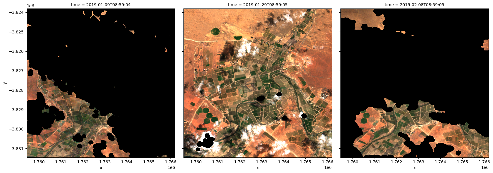
Tracez les pas de temps en vraies couleurs
Pour visualiser les données, utilisez la fonction utilitaire « rgb » préchargée pour tracer une image en vraies couleurs pour une série d’intervalles de temps. Les zones noires indiquent les endroits où les nuages ou autres pixels non valides de l’image ont été définis sur « -999 » pour indiquer l’absence de données.
Le code ci-dessous tracera trois étapes temporelles de la série temporelle que nous venons de charger.
[6]:
# Set the timesteps to visualise
timesteps = [1, 5, 7]

# Generate RGB plots at each timestep
rgb(ds, index=timesteps)
/opt/venv/lib/python3.12/site-packages/odc/algo/_masking.py:425: FutureWarning: `binary_opening` is deprecated since version 0.26 and will be removed in version 0.28. Use `skimage.morphology.opening` instead.
  mask = op(mask, _disk(radius, mask.ndim))
/opt/venv/lib/python3.12/site-packages/odc/algo/_masking.py:425: FutureWarning: `binary_dilation` is deprecated since version 0.26 and will be removed in version 0.28. Use `skimage.morphology.dilation` instead. Note the lack of mirroring for non-symmetric footprints (see docstring notes).
  mask = op(mask, _disk(radius, mask.ndim))
/opt/venv/lib/python3.12/site-packages/rasterio/warp.py:385: NotGeoreferencedWarning: Dataset has no geotransform, gcps, or rpcs. The identity matrix will be returned.
  dest = _reproject(
/opt/venv/lib/python3.12/site-packages/odc/algo/_masking.py:425: FutureWarning: `binary_opening` is deprecated since version 0.26 and will be removed in version 0.28. Use `skimage.morphology.opening` instead.
  mask = op(mask, _disk(radius, mask.ndim))
/opt/venv/lib/python3.12/site-packages/odc/algo/_masking.py:425: FutureWarning: `binary_dilation` is deprecated since version 0.26 and will be removed in version 0.28. Use `skimage.morphology.dilation` instead. Note the lack of mirroring for non-symmetric footprints (see docstring notes).
  mask = op(mask, _disk(radius, mask.ndim))
Générer une géomédiane
Comme vous pouvez le voir ci-dessus, la plupart des images satellites auront au moins quelques zones masquées en raison de nuages ou d’autres interférences entre le satellite et le sol. L’exécution de la fonction geomedian_with_mads générera un composite géomédian en combinant toutes les observations de notre xarray.Dataset en une seule image complète (ou presque complète) représentant la médiane géométrique de la période.
Remarque : étant donné que nos données ont été chargées paresseusement avec « dask », l’algorithme géomédian lui-même ne sera pas déclenché tant que nous n’aurons pas appelé la méthode « .compute() » à l’étape suivante.
[7]:
# geomedian = int_geomedian(ds)
geomedian = geomedian_with_mads(ds,
                               compute_mads=False,
                               compute_count=False,
                               reshape_strategy="yxbt"  # Instead of default "mem"
                               )
Exécuter le calcul
La méthode « .compute() » déclenchera le calcul de l’algorithme géomédian ci-dessus. L’exécution prendra environ quelques minutes ; consultez le « tableau de bord dask » pour vérifier la progression.
[8]:
%%time
geomedian = geomedian.compute()
/opt/venv/lib/python3.12/site-packages/odc/algo/_masking.py:425: FutureWarning: `binary_opening` is deprecated since version 0.26 and will be removed in version 0.28. Use `skimage.morphology.opening` instead.
  mask = op(mask, _disk(radius, mask.ndim))
/opt/venv/lib/python3.12/site-packages/odc/algo/_masking.py:425: FutureWarning: `binary_dilation` is deprecated since version 0.26 and will be removed in version 0.28. Use `skimage.morphology.dilation` instead. Note the lack of mirroring for non-symmetric footprints (see docstring notes).
  mask = op(mask, _disk(radius, mask.ndim))
CPU times: user 2.83 s, sys: 338 ms, total: 3.17 s
Wall time: 1min 7s
Si nous imprimons notre résultat, vous verrez que la dimension « temps » a maintenant été supprimée et qu’il nous reste une seule image qui représente la médiane géométrique de toutes les images satellites de notre série temporelle initiale :
[9]:
geomedian
[9]:
<xarray.Dataset> Size: 3MB
Dimensions:  (y: 765, x: 677)
Coordinates:
  * y        (y) float64 6kB -3.824e+06 -3.824e+06 ... -3.831e+06 -3.831e+06
  * x        (x) float64 5kB 1.759e+06 1.759e+06 ... 1.766e+06 1.766e+06
Data variables:
    green    (y, x) uint16 1MB 1243 1303 1330 1320 1240 ... 1496 1478 1384 1294
    red      (y, x) uint16 1MB 1900 1992 2036 2018 1889 ... 2533 2525 2362 2235
    blue     (y, x) uint16 1MB 732 777 799 788 736 693 ... 894 912 898 824 773
Attributes:
    units:         1
    nodata:        0
    crs:           EPSG:6933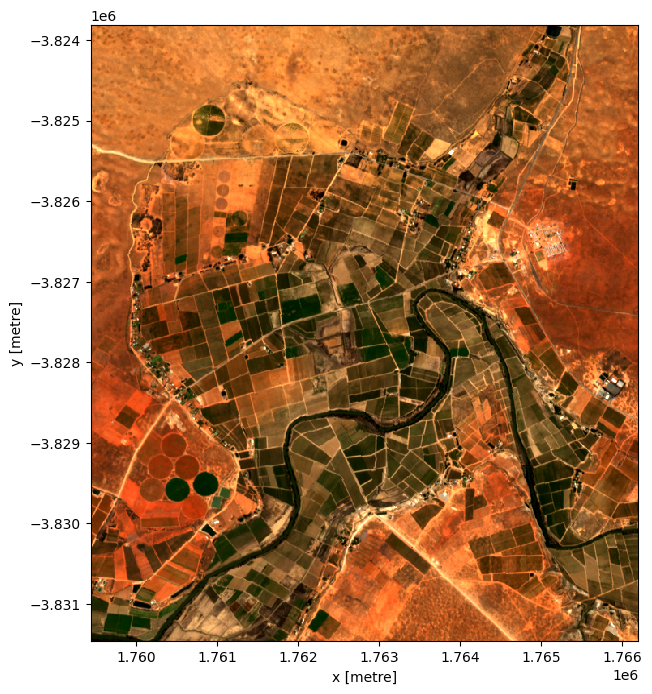
grid_mapping: spatial_refTracer le composite géomédian
En traçant le résultat, nous pouvons voir que l’image géomédiane est beaucoup plus complète que n’importe laquelle des images individuelles. Nous pouvons également utiliser ces données dans l’analyse en aval, car les relations entre les bandes spectrales sont maintenues par la statistique médiane géométrique.
[10]:
# Plot the result
rgb(geomedian, size=8)
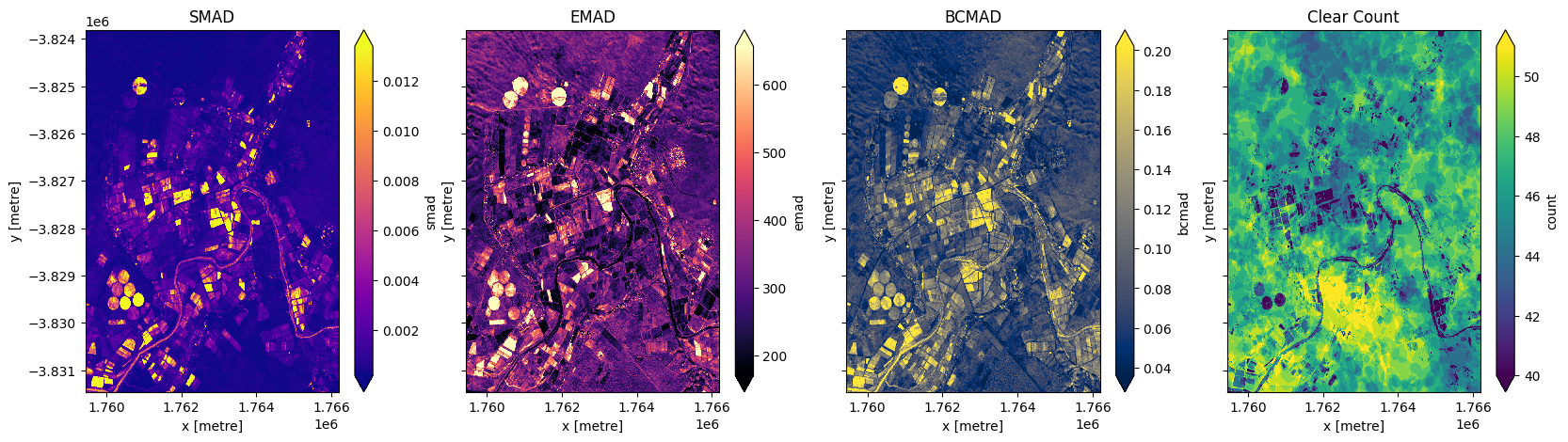
Générer des écarts absolus médians
En plus d’exécuter un composite géomédian, qui renverra les observations médianes pour chaque bande, nous pouvons également calculer la variation que subit chaque pixel au cours de la série temporelle. La fonction geomedian_with_mads renvoie trois mesures de variabilité : l’écart absolu médian spectral (smad), l’écart absolu médian euclidien (emad) et l’écart absolu médian Bray-Curtis (bcmad).
Pour calculer les trois mesures de variabilité, transmettez simplement « compute_mads=True » à la fonction « geomedian_with_mads ». Cette fonction prend également en charge le renvoi de « count », qui renvoie le nombre d’observations claires pour chaque pixel.
[11]:
geomads = geomedian_with_mads(ds,
                              compute_mads=True,
                              compute_count=True,
                              reshape_strategy="yxbt"  # Instead of default "mem"
                             )

geomads = geomads.compute()
print(geomads)
<xarray.Dataset> Size: 10MB
Dimensions:  (y: 765, x: 677)
Coordinates:
  * y        (y) float64 6kB -3.824e+06 -3.824e+06 ... -3.831e+06 -3.831e+06
  * x        (x) float64 5kB 1.759e+06 1.759e+06 ... 1.766e+06 1.766e+06
Data variables:
    green    (y, x) uint16 1MB 1243 1303 1330 1320 1240 ... 1496 1478 1384 1294
    red      (y, x) uint16 1MB 1900 1992 2036 2018 1889 ... 2533 2525 2362 2235
    blue     (y, x) uint16 1MB 732 777 799 788 736 693 ... 894 912 898 824 773
    smad     (y, x) float32 2MB 0.0001308 0.0001117 ... 0.0002928 0.0002812
    emad     (y, x) float32 2MB 824.4 771.3 780.8 ... 913.3 1.12e+03 1.326e+03
    bcmad    (y, x) float32 2MB 0.1552 0.143 0.1391 ... 0.1322 0.1671 0.1991
    count    (y, x) uint16 1MB 72 72 72 72 72 72 72 72 ... 72 72 72 72 72 72 72
Attributes:
    units:         1
    nodata:        0
    crs:           EPSG:6933
    grid_mapping:  spatial_ref
Tracer les écarts absolus médians et effacer le décompte
[12]:
fig,ax=plt.subplots(1,4, sharey=True, figsize=(20,5))
geomads['smad'].plot(ax=ax[0], cmap='plasma', robust=True)
geomads['emad'].plot(ax=ax[1], cmap='magma', robust=True)
geomads['bcmad'].plot(ax=ax[2], cmap='cividis', robust=True)
geomads['count'].plot(ax=ax[3], cmap='viridis', robust=True)
ax[0].set_title('SMAD')
ax[1].set_title('EMAD')
ax[2].set_title('BCMAD')
ax[3].set_title('Clear Count');
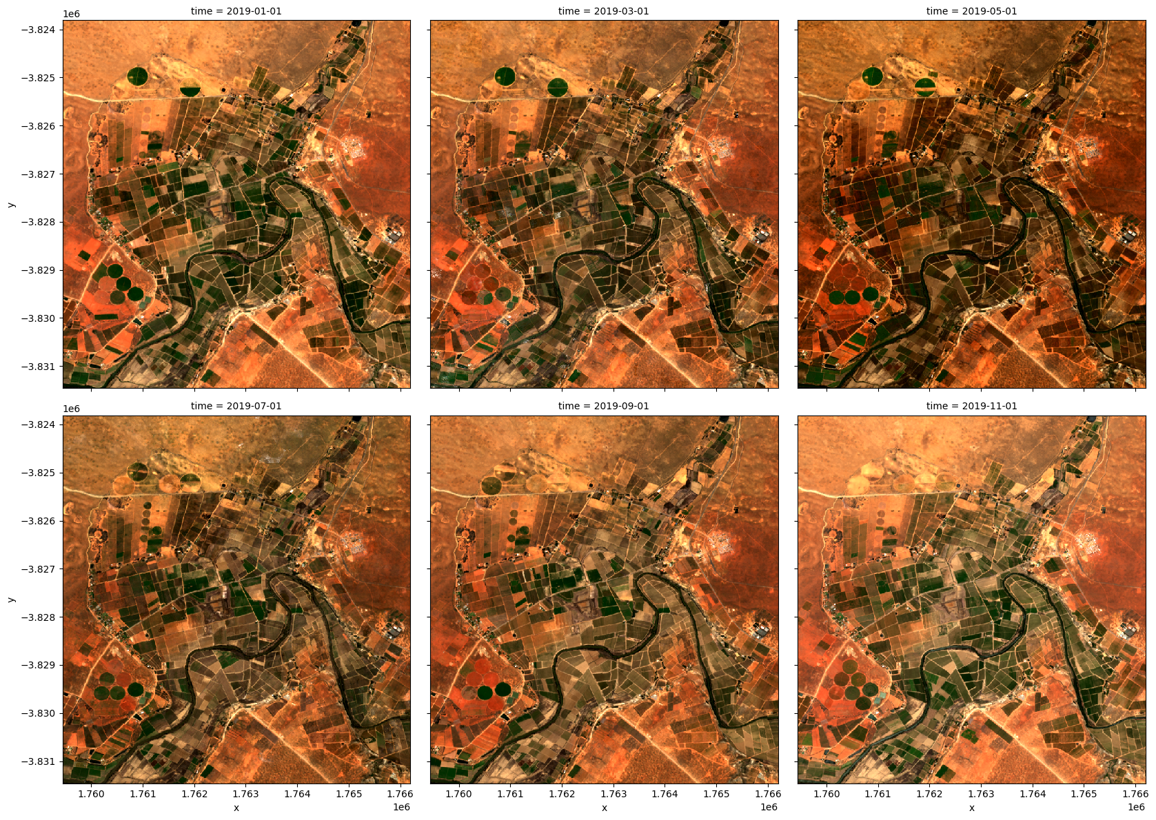
Exécution de GeoMADs sur des séries chronologiques groupées ou rééchantillonnées
mean et median sont exécutées sur des données de séries chronologiques qui ont été rééchantillonnées ou groupées.Rééchantillonnage
Nous allons d’abord diviser la série temporelle en groupes souhaités. Le rééchantillonnage peut être utilisé pour créer un nouvel ensemble de temps à intervalles réguliers :
groupé = da_scaled.resample(time=1M)« nD » - nombre de jours (par exemple, « 7D » pour sept jours)
« nM » - nombre de mois (par exemple, « 6M » pour six mois)
« nY » - nombre d’années (par exemple, « 2Y » pour deux ans)
Grouper par
Le regroupement fonctionne en examinant une partie de la date, mais en ignorant les autres parties. Par exemple, « time.month » regrouperait toutes les données de janvier, quelle que soit l’année à laquelle elles appartiennent.
groupé = da_scaled.groupby('time.month')``”time.day””` - regroupe par jour du mois (1-31)
'time.dayofyear'- regroupe par jour de l’année (1-365)'time.week'- groupes par semaine (1-52)'time.month'- groupes par mois (1-12)'time.season'- regroupe en saisons de 3 mois :'DJF'Décembre, Janvier, Février'MAM'mars, avril, mai« JJA » juin, juillet, août
'SON'Septembre, octobre, novembre
'time.year'- regroupe par année
Ici, nous allons rééchantillonner en trois groupes de deux mois (« 2M »), le groupe commençant au début du mois (représenté par le « S » à la fin).
[13]:
grouped = ds.resample(time='2MS')
grouped
[13]:
<DatasetResample, grouped over 1 grouper(s), 6 groups in total:
    '__resample_dim__': TimeResampler('__resample_dim__'), 6/6 groups with labels 2019-01-01, ..., 2019-11-01>
Nous allons maintenant appliquer la fonction « geomedian_with_mads » à chaque groupe rééchantillonné en utilisant la méthode « map ».
Au lieu d’appeler « geomedian_with_mads(ds) » sur l’ensemble du tableau, nous passons la fonction « geomedian_with_mads » à « map » pour l’appliquer séparément à chaque groupe rééchantillonné.
[14]:
geomedian_grouped = grouped.map(geomedian_with_mads, reshape_strategy="yxbt") # Instead of default "mem"
Nous pouvons maintenant déclencher le calcul et observer la progression à l’aide du tableau de bord Dask.
[15]:
geomedian_grouped = geomedian_grouped.compute()
Nous pouvons tracer les géomédianes de sortie et voir l’évolution du paysage au cours de l’année :
[16]:
rgb(geomedian_grouped, col='time', col_wrap=3)
Avancé : GeoMADs sur données Landsat
Ci-dessous, nous calculons les GeoMADs à l’aide de Landsat 8. Pour que le GeoMAD corresponde à Sentinel-2, nous devons franchir une étape supplémentaire. Les données de réflectance de surface Landsat sont mises à l’échelle de 0 à 1, tandis que les données Sentinel-2 sont mises à l’échelle de 0 à 10 000. Pour que les deux ensembles de données correspondent, nous devons multiplier les bandes Landsat par 10 000 (cela fera que les geoMADs produits dans ce bloc-notes correspondront à l’ensemble de données « gm_ls8_annual » disponible dans le datacube). Les bandes « bcmad » et « smad » n’ont pas besoin d’être multipliées par 10 000.
[17]:
# Load available data for Landsat 8
ds = load_ard(dc=dc,
              x=lon_range,
              y=lat_range,
              time=('2019-01', '2019-12'),
              measurements=['green','red','blue'],
              products=['ls8_sr'],
              dask_chunks={'x':1000, 'y':1000},
              mask_filters=(['opening',3], ['dilation',3]), #improve cloud mask
              resolution=(-30,30),
              group_by='solar_day',
              output_crs='EPSG:6933'
             )

# Print output data
print(ds)
Using pixel quality parameters for USGS Collection 2
Finding datasets
    ls8_sr
Applying morphological filters to pq mask (['opening', 3], ['dilation', 3])
Applying pixel quality/cloud mask
Re-scaling Landsat C2 data
Returning 23 time steps as a dask array
<xarray.Dataset> Size: 16MB
Dimensions:      (time: 23, y: 256, x: 226)
Coordinates:
  * time         (time) datetime64[ns] 184B 2019-01-08T08:40:51.853294 ... 20...
  * y            (y) float64 2kB -3.824e+06 -3.824e+06 ... -3.831e+06 -3.831e+06
  * x            (x) float64 2kB 1.759e+06 1.759e+06 ... 1.766e+06 1.766e+06
    spatial_ref  int32 4B 6933
Data variables:
    green        (time, y, x) float32 5MB dask.array<chunksize=(1, 256, 226), meta=np.ndarray>
    red          (time, y, x) float32 5MB dask.array<chunksize=(1, 256, 226), meta=np.ndarray>
    blue         (time, y, x) float32 5MB dask.array<chunksize=(1, 256, 226), meta=np.ndarray>
Attributes:
    crs:           EPSG:6933
    grid_mapping:  spatial_ref
/opt/venv/lib/python3.12/site-packages/odc/algo/_masking.py:425: FutureWarning: `binary_opening` is deprecated since version 0.26 and will be removed in version 0.28. Use `skimage.morphology.opening` instead.
  mask = op(mask, _disk(radius, mask.ndim))
/opt/venv/lib/python3.12/site-packages/odc/algo/_masking.py:425: FutureWarning: `binary_dilation` is deprecated since version 0.26 and will be removed in version 0.28. Use `skimage.morphology.dilation` instead. Note the lack of mirroring for non-symmetric footprints (see docstring notes).
  mask = op(mask, _disk(radius, mask.ndim))
/opt/venv/lib/python3.12/site-packages/deafrica_tools/datahandling.py:565: FutureWarning: In a future version of xarray the default value for compat will change from compat='no_conflicts' to compat='override'. This is likely to lead to different results when combining overlapping variables with the same name. To opt in to new defaults and get rid of these warnings now use `set_options(use_new_combine_kwarg_defaults=True) or set compat explicitly.
  ds = xr.merge([ds_data, ds_masks])
Calculer les GeoMADs sur les données Landsat
[18]:
geomads = geomedian_with_mads(ds,  reshape_strategy="yxbt", compute_mads=True, compute_count=True).compute() # Instead of default "mem"
print(geomads)
<xarray.Dataset> Size: 2MB
Dimensions:  (y: 256, x: 226)
Coordinates:
  * y        (y) float64 2kB -3.824e+06 -3.824e+06 ... -3.831e+06 -3.831e+06
  * x        (x) float64 2kB 1.759e+06 1.759e+06 ... 1.766e+06 1.766e+06
Data variables:
    green    (y, x) float32 231kB 0.1419 0.1439 0.1352 ... 0.1597 0.1509 0.1506
    red      (y, x) float32 231kB 0.2158 0.2185 0.2056 ... 0.2627 0.2512 0.2384
    blue     (y, x) float32 231kB 0.07643 0.07741 0.07278 ... 0.07561 0.07653
    smad     (y, x) float32 231kB 1.878e-05 3.331e-05 ... 0.0002164 0.0003216
    emad     (y, x) float32 231kB 0.03394 0.02932 0.03075 ... 0.02122 0.01755
    bcmad    (y, x) float32 231kB 0.05951 0.05521 0.0572 ... 0.03528 0.03135
    count    (y, x) uint16 116kB 15 15 14 14 14 14 14 ... 14 14 14 14 14 14 14
Attributes:
    units:         1
    nodata:        0
    crs:           EPSG:6933
    grid_mapping:  spatial_ref
Multipliez les bandes par 10 000 pour correspondre à Sentinel-2
[19]:
exclude = ['bcmad', 'smad', 'count']

for band in geomads.data_vars:
    if band not in exclude:
        geomads[band] = geomads[band]*10000
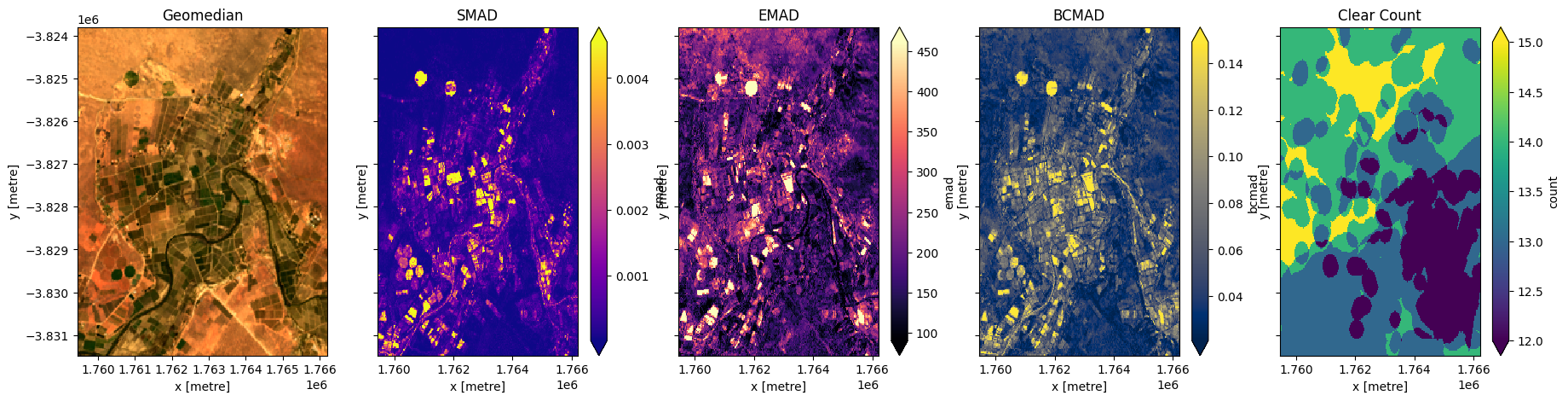
Tracer le Landsat GeoMAD
[20]:
fig,ax=plt.subplots(1,5, sharey=True, figsize=(22,5))
rgb(geomads, ax=ax[0])
geomads['smad'].plot(ax=ax[1], cmap='plasma', robust=True)
geomads['emad'].plot(ax=ax[2], cmap='magma', robust=True)
geomads['bcmad'].plot(ax=ax[3], cmap='cividis', robust=True)
geomads['count'].plot(ax=ax[4], cmap='viridis', robust=True)
ax[0].set_title('Geomedian')
ax[1].set_title('SMAD')
ax[2].set_title('EMAD')
ax[3].set_title('BCMAD')
ax[4].set_title('Clear Count');
Informations Complémentaires
Licence : Le code de ce carnet est sous licence Apache, version 2.0 <https://www.apache.org/licenses/LICENSE-2.0>. Les données de Digital Earth Africa sont sous licence Creative Commons par attribution 4.0 <https://creativecommons.org/licenses/by/4.0/>.
Contact : Si vous avez besoin d’aide, veuillez poster une question sur le canal Slack Open Data Cube <http://slack.opendatacube.org/>`__ ou sur le GIS Stack Exchange en utilisant la balise open-data-cube (vous pouvez consulter les questions posées précédemment ici). Si vous souhaitez signaler un problème avec ce bloc-notes, vous pouvez en déposer un sur Github.
Version de Datacube compatible :
[21]:
print(datacube.__version__)
1.9.13
Dernier test :
[22]:
from datetime import datetime
datetime.today().strftime('%Y-%m-%d')
[22]:
'2026-04-08'