Générer des images composites

• Produits utilisés : s2_l2a

Mots clés données utilisées ; sentinelle-2, indice de bande ; NDVI, analyse ; séries chronologiques, analyse ; composites

Aperçu

Les images individuelles de télédétection peuvent être affectées par des données bruyantes, notamment des nuages, des ombres de nuages et de la brume. Pour produire des images plus nettes qui peuvent être comparées plus facilement dans le temps, nous pouvons créer des images « récapitulatives » ou « composites » qui combinent plusieurs images en une seule.

Certaines méthodes de génération de composites incluent l’estimation des valeurs de pixels « médianes », « moyennes », « minimales » ou « maximales » dans une image. Il faut être prudent avec ces valeurs, car elles ne préservent pas nécessairement les relations spectrales entre les bandes. Pour savoir comment générer un composite qui préserve ces relations, consultez le bloc-notes « Génération de composites géomédians <Generating_geomedian_composites.ipynb> ».

Description

Ce bloc-notes montre comment générer un certain nombre de composites différents à partir d’images satellites et décrit les utilisations de chacun. Plus précisément, ce bloc-notes montre comment générer :

1. Composites médians

2. Composites moyens

3. Composites minimum et maximum

4. Composites au temps le plus proche

---

Commencer

Pour exécuter cette analyse, exécutez toutes les cellules du bloc-notes, en commençant par la cellule « Charger les packages ».

Charger des paquets

Importez les packages Python utilisés pour l’analyse.

%matplotlib inline

import datacube
import matplotlib.pyplot as plt
import xarray as xr
import geopandas as gpd
from datacube.utils.geometry import Geometry

from deafrica_tools.plotting import rgb
from deafrica_tools.datahandling import load_ard, mostcommon_crs, first, last, nearest
from deafrica_tools.bandindices import calculate_indices
from deafrica_tools.areaofinterest import define_area

Se connecter au datacube

Connectez-vous au datacube pour que nous puissions accéder aux données de DE Africa. Le paramètre « app » est un nom unique pour l’analyse qui est basé sur le nom du fichier du notebook.

dc = datacube.Datacube(app='Generating_composites')

Charger les données Sentinel-2

Ici, nous chargeons une série chronologique d’images satellites Sentinel-2 masquées par des nuages via l’API datacube à l’aide de la fonction load_ard.

Pour définir la zone d’intérêt, deux méthodes sont disponibles :

1. En spécifiant la latitude, la longitude et la zone tampon. Cette méthode nécessite que vous saisissiez la latitude centrale, la longitude centrale et la valeur de la zone tampon en degrés carrés autour du point central que vous souhaitez analyser. Par exemple, « lat = 10,338 », « lon = -1,055 » et « buffer = 0,1 » sélectionneront une zone avec un rayon de 0,1 degré carré autour du point avec les coordonnées (10,338, -1,055).

2. By uploading a polygon as a GeoJSON or Esri Shapefile. If you choose this option, you will need to upload the geojson or ESRI shapefile into the Sandbox using Upload Files button in the top left corner of the Jupyter Notebook interface. ESRI shapefiles must be uploaded with all the related files (.cpg, .dbf, .shp, .shx). Once uploaded, you can use the shapefile or geojson to define the area of interest. Remember to update the code to call the file you have uploaded.

Pour utiliser l’une de ces méthodes, vous pouvez décommenter la ligne de code concernée et commenter l’autre. Pour commenter une ligne, ajoutez le symbole "#" avant le code que vous souhaitez commenter. Par défaut, la première option qui définit l’emplacement à l’aide de la latitude, de la longitude et du tampon est utilisée.

# Set the area of interest

# Method 1: Specify the latitude, longitude, and buffer
aoi = define_area(lat=14.970, lon=-4.127, buffer=0.075)

# Method 2: Use a polygon as a GeoJSON or Esri Shapefile.
# aoi = define_area(vector_path='aoi.shp')

#Create a geopolygon and geodataframe of the area of interest
geopolygon = Geometry(aoi["features"][0]["geometry"], crs="epsg:4326")
geopolygon_gdf = gpd.GeoDataFrame(geometry=[geopolygon], crs=geopolygon.crs)

# Get the latitude and longitude range of the geopolygon
lat_range = (geopolygon_gdf.total_bounds[1], geopolygon_gdf.total_bounds[3])
lon_range = (geopolygon_gdf.total_bounds[0], geopolygon_gdf.total_bounds[2])

# Create a reusable query
query = {
    'x': lon_range,
    'y': lat_range,
    'time': ('2019'),
    'measurements': ['green', 'red', 'blue', 'nir'],
    'resolution': (-20, 20),
    'group_by': 'solar_day'
}

# Identify the most common projection system in the input query
output_crs = mostcommon_crs(dc=dc, product='s2_l2a', query=query)

# Load available data
ds = load_ard(dc=dc,
              products=['s2_l2a'],
              output_crs=output_crs,
              **query)

# Print output data
print(ds)

Using pixel quality parameters for Sentinel 2
Finding datasets
    s2_l2a
Applying pixel quality/cloud mask
Loading 73 time steps
<xarray.Dataset>
Dimensions:      (time: 73, y: 834, x: 811)
Coordinates:
  * time         (time) datetime64[ns] 2019-01-03T10:56:58 ... 2019-12-29T10:...
  * y            (y) float64 1.664e+06 1.664e+06 ... 1.647e+06 1.647e+06
  * x            (x) float64 3.707e+05 3.707e+05 ... 3.869e+05 3.869e+05
    spatial_ref  int32 32630
Data variables:
    green        (time, y, x) float32 2.057e+03 2.118e+03 ... 1.451e+03 1.66e+03
    red          (time, y, x) float32 2.519e+03 2.603e+03 ... 1.59e+03 1.727e+03
    blue         (time, y, x) float32 1.408e+03 1.505e+03 ... 742.0 838.0
    nir          (time, y, x) float32 3.623e+03 3.664e+03 ... 4.147e+03
Attributes:
    crs:           epsg:32630
    grid_mapping:  spatial_ref

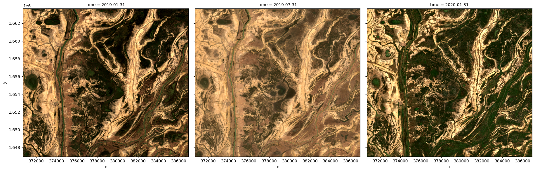
Tracez les pas de temps en vraies couleurs

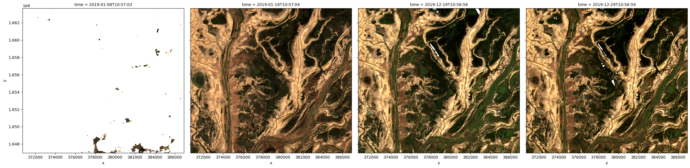
Pour visualiser les données, utilisez la fonction utilitaire « rgb » préchargée pour tracer une image en vraies couleurs pour une série d’intervalles de temps. Les zones blanches indiquent les endroits où les nuages ou autres pixels non valides de l’image ont été masqués.

Le code ci-dessous tracera quatre pas de temps de la série chronologique que nous venons de charger.

# Set the timesteps to visualise
timesteps = [1, 3, -3, -1]

# Generate RGB plots at each timestep
rgb(ds, index=timesteps)

/usr/local/lib/python3.10/dist-packages/matplotlib/cm.py:478: RuntimeWarning: invalid value encountered in cast
  xx = (xx * 255).astype(np.uint8)

Composites médians

L’une des principales raisons de générer une image composite est de remplacer les pixels classés comme nuages par des valeurs réalistes issues des données disponibles. Cela permet d’obtenir une image qui ne contient aucun nuage. Dans le cas d’une image composite médiane, chaque pixel est sélectionné pour avoir la valeur médiane (ou moyenne) parmi toutes les valeurs possibles.

Il convient d’être prudent lors de l’utilisation de ces composites pour l’analyse, car les relations entre les bandes spectrales ne sont pas préservées. Ces composites sont également affectés par la période sur laquelle ils sont générés. Par exemple, la valeur médiane des pixels d’une seule saison peut être différente de la valeur médiane de l’année entière.

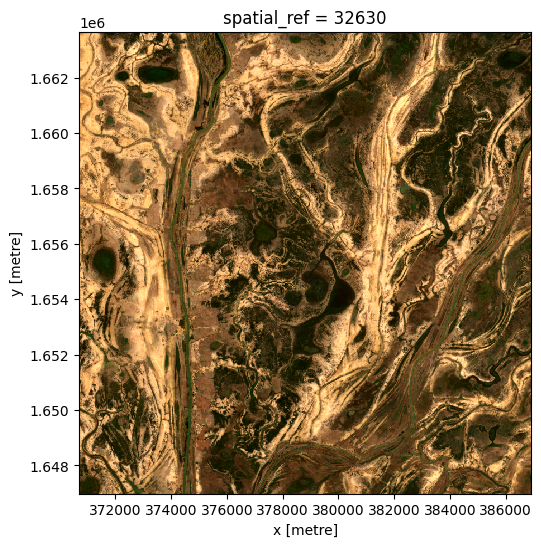
Générer un composite unique à partir de toutes les données

Pour générer un composite médian unique, nous utilisons la méthode « xarray.median », en spécifiant « time » comme dimension sur laquelle calculer la médiane.

# Compute a single median from all data
ds_median = ds.median('time')

# View the resulting median
rgb(ds_median, bands=['red', 'green', 'blue'])

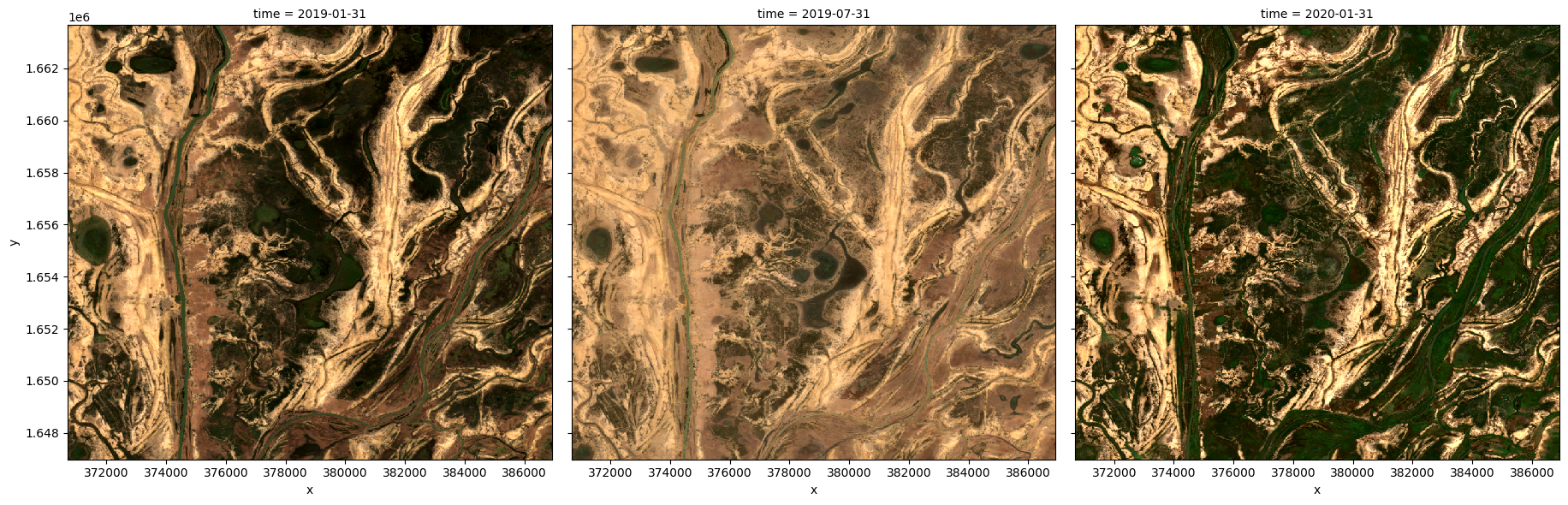
Générer plusieurs composites en fonction de la durée

Plutôt que d’utiliser toutes les données pour générer une seule médiane composite, il est possible d’utiliser la méthode « xarray.resample » pour regrouper les données en périodes plus petites et générer des médianes pour chacune d’entre elles. Voici quelques options de rééchantillonnage : * « nD » - nombre de jours (par exemple, « 7D » pour sept jours) * « nM » - nombre de mois (par exemple, « 6M » pour six mois) * « nY » - nombre d’années (par exemple, « 2Y » pour deux ans)

Si la zone est particulièrement nuageuse pendant l’une des périodes, il se peut que des pixels masqués apparaissent toujours dans la médiane. Cela sera vrai si ce pixel est toujours masqué.

# Generate a median by binning data into six-monthly time-spans
ds_resampled_median = ds.resample(time='6M').median('time')

# View the resulting medians
rgb(ds_resampled_median, bands=['red', 'green', 'blue'], col='time')

/usr/local/lib/python3.10/dist-packages/matplotlib/cm.py:478: RuntimeWarning: invalid value encountered in cast
  xx = (xx * 255).astype(np.uint8)

Grouper par

Similairement au rééchantillonnage, le regroupement fonctionne en examinant une partie de la date, mais en ignorant les autres parties. Par exemple, « time.month » regrouperait toutes les données de janvier, quelle que soit l’année à laquelle elles appartiennent.

Voici quelques exemples : * 'time.day' - regroupe par jour du mois (1-31) * 'time.dayofyear' - regroupe par jour de l’année (1-365) * 'time.week' - regroupe par semaine (1-52) * 'time.month' - regroupe par mois (1-12) * 'time.season' - regroupe par saisons de 3 mois : - 'DJF' décembre, janvier, février - 'MAM' mars, avril, mai - 'JJA' juin, juillet, août - 'SON' septembre, octobre, novembre * 'time.year' - regroupe par année

# Generate a median by binning data into six-monthly time-spans
ds_groupby_season = ds.groupby('time.season').median()

# View the resulting medians
rgb(ds_groupby_season, bands=['red', 'green', 'blue'], col='season')

/usr/local/lib/python3.10/dist-packages/matplotlib/cm.py:478: RuntimeWarning: invalid value encountered in cast
  xx = (xx * 255).astype(np.uint8)

Composites moyens

Les composites moyens impliquent de prendre la valeur moyenne de chaque pixel, plutôt que la valeur médiane comme c’est le cas pour un composite médian. Contrairement à la médiane, le composite moyen peut contenir des valeurs de pixels qui ne faisaient pas partie de l’ensemble de données d’origine. Il convient d’être prudent lors de l’interprétation de ces images, car les valeurs extrêmes (comme un nuage non masqué) peuvent fortement affecter la moyenne.

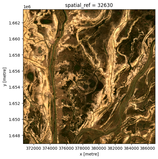
Générer un composite unique à partir de toutes les données

Pour générer une moyenne composite unique, nous utilisons la méthode « xarray.mean », en spécifiant « time » comme dimension sur laquelle calculer la moyenne.

Remarque : s’il n’existe aucune valeur valide pour un pixel donné, vous pouvez voir l’avertissement : « RuntimeWarning : moyenne d’une tranche vide ». Le composite sera toujours généré, mais il pourra contenir des zones vides.

# Compute a single mean from all data
ds_mean = ds.mean('time')

# View the resulting mean
rgb(ds_mean, bands=['red', 'green', 'blue'])

Générer plusieurs composites en fonction de la durée

Comme pour la médiane composite, il est possible d’utiliser la méthode « xarray.resample » pour regrouper les données en intervalles de temps plus petits et générer des moyennes pour chacun d’entre eux. Voir la section précédente pour quelques exemples de rééchantillonnage d’intervalles de temps.

Remarque : si vous recevez l’avertissement « RuntimeWarning : moyenne de la tranche vide », cela signifie simplement que pour l’un de vos groupes, il y avait au moins un pixel contenant toutes les valeurs « nan ».

# Generate a mean by binning data into six-monthly time-spans
ds_resampled_mean = ds.resample(time='6M').mean('time')

# View the resulting medians
rgb(ds_resampled_mean, bands=['red', 'green', 'blue'], col='time')

/usr/local/lib/python3.10/dist-packages/matplotlib/cm.py:478: RuntimeWarning: invalid value encountered in cast
  xx = (xx * 255).astype(np.uint8)

Composites minimum et maximum

Ces composites peuvent être utiles pour identifier un comportement extrême dans une collection d’images satellites.

Par exemple, la comparaison des composites maximum et minimum pour un indice de bande donné pourrait aider à identifier les zones qui adoptent une large gamme de valeurs, ce qui peut indiquer des zones qui présentent une forte variabilité sur la chronologie du composite.

Pour démontrer cela, nous commençons par calculer l’indice de végétation par différence normalisée (NDVI) pour nos données, qui peut ensuite être utilisé pour générer les composites maximum et minimum.

# Start by calculating NDVI
ds = calculate_indices(ds, index='NDVI', satellite_mission='s2')

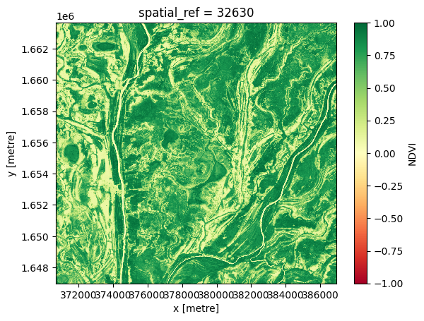
Composite maximal

Pour générer un composite maximum unique, nous utilisons la méthode « xarray.max », en spécifiant « time » comme dimension sur laquelle calculer le maximum.

# Compute the maximum composite
ds_max = ds.NDVI.max('time')

# View the resulting composite
ds_max.plot(vmin=-1, vmax=1, cmap='RdYlGn');

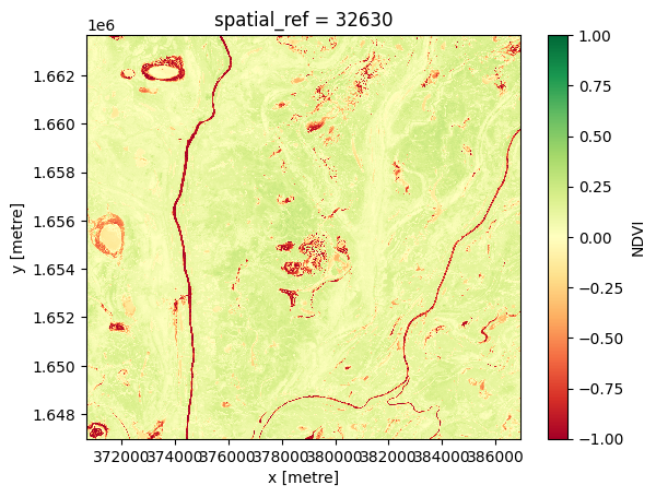
Composite minimum

Pour générer un composite minimum unique, nous utilisons la méthode « xarray.min », en spécifiant « time » comme dimension sur laquelle calculer le minimum.

# Compute the minimum composite
ds_min = ds.NDVI.min('time')

# View the resulting composite
ds_min.plot(vmin=-1, vmax=1, cmap='RdYlGn');

Composites au temps le plus proche

Pour obtenir une image à un moment donné, il manque souvent des données, en raison des nuages et d’autres masquages. Nous pouvons combler ces lacunes en utilisant des données des périodes environnantes.

Pour générer ces images, nous pouvons utiliser les fonctions personnalisées first, last et nearest du module deafrica.datahandling.

Vous pouvez également utiliser les méthodes intégrées .first() et .last() lors de l’exécution de groupby et resample comme décrit ci-dessus. Elles sont décrites dans la documentation xarray sur les données groupées.

Composite le plus récent

Parfois, nous souhaitons déterminer à quoi ressemble le paysage en examinant l’image la plus récente. Si nous regardons la dernière image de notre ensemble de données, nous pouvons voir qu’il manque des données au centre de la dernière image.

# Plot the last image in time
rgb(ds, index=[-1])

/usr/local/lib/python3.10/dist-packages/matplotlib/cm.py:478: RuntimeWarning: invalid value encountered in cast
  xx = (xx * 255).astype(np.uint8)

Nous pouvons calculer la quantité de données manquantes dans cette image la plus récente

last_blue_image = ds.blue.isel(time=-1)

precent_valid_data = float(last_blue_image.count() / last_blue_image.size) * 100
print(f"The last image contains {precent_valid_data:.2f}% data.")

The last image contains 99.79% data.

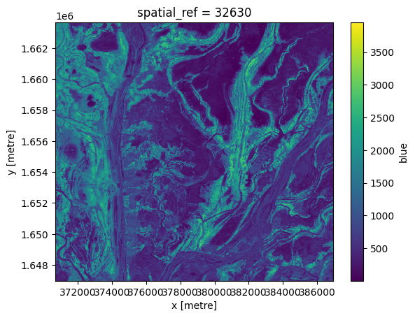
Afin de combler les lacunes et de produire une image complète montrant l’acquisition satellite la plus récente pour chaque pixel, nous pouvons exécuter la fonction « last » sur l’un des tableaux.

last_blue = last(ds.blue, dim='time')
last_blue.plot();

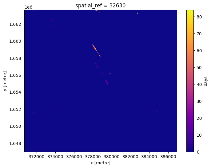
Pour voir à quel point chaque pixel est récent, nous pouvons comparer l’âge des pixels avec la dernière valeur dont nous disposons.

Ici, nous pouvons voir que la plupart des pixels proviennent de la dernière tranche de temps, même si certains sont beaucoup plus anciens.

# Identify lastest time in our data
last_time = last_blue.time.max()

# Compare the timestamps and convert them to number of days for plotting.
num_days_old = (last_time - last_blue.time).dt.days
num_days_old.plot(cmap='plasma', size=6);

Nous pouvons exécuter cette méthode sur toutes les bandes. Cependant, nous voulons uniquement les pixels qui ont des données dans chaque bande. Sur les bords d’un passage satellite, certaines bandes n’ont pas de données.

Pour nous débarrasser des pixels avec des données manquantes, nous allons convertir l’ensemble de données en tableau et sélectionner uniquement les pixels avec des données dans toutes les bandes.

#Convert to array
da = ds.to_array(dim='variable')
#create a mask where data has no-data
no_data_mask = da.isnull().any(dim='variable')
#mask out regions where there is no-data
da = da.where(~no_data_mask)

Nous pouvons maintenant exécuter la fonction « last » sur le tableau, puis le transformer à nouveau en un ensemble de données.

da_latest = last(da, dim='time')

ds_latest = da_latest.to_dataset(dim='variable').drop_dims('variable')

# View the resulting composite
rgb(ds_latest, bands=['red', 'green', 'blue'])

Avant et après les composites

Il est souvent utile de visualiser des images avant et après un événement, pour voir le changement qui s’est produit.

Pour générer un composite de chaque côté d’un événement, nous pouvons diviser l’ensemble de données au fil du temps.

Nous pouvons alors visualiser la « dernière » image composite avant l’événement, et la « première » image composite après l’événement.

# Dates here are inclusive. Use None to not set a start or end of the range.
before_event = slice(None, '2019-06-01')
after_event = slice('2019-06-03', None)

# Select the time period and run the last() or first() function on every band.
da_before = last(da.sel(time=before_event), dim='time')
da_after = first(da.sel(time=after_event), dim='time')

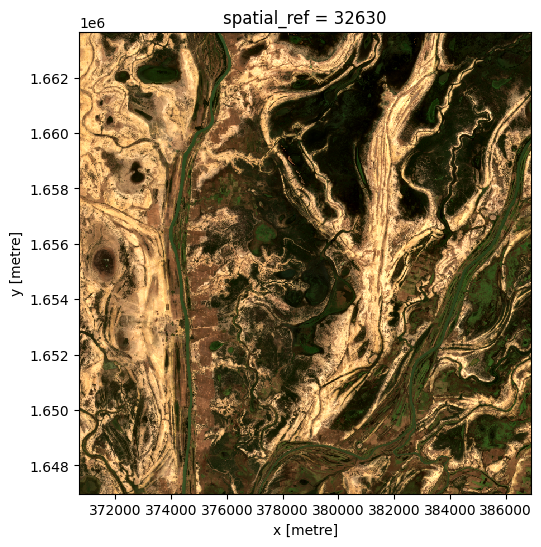
L’image composite avant l’événement, jusqu’au 01/06/2019 :

ds_before = da_before.to_dataset(dim='variable').drop_dims('variable')

rgb(ds_before, bands=['red', 'green', 'blue'])

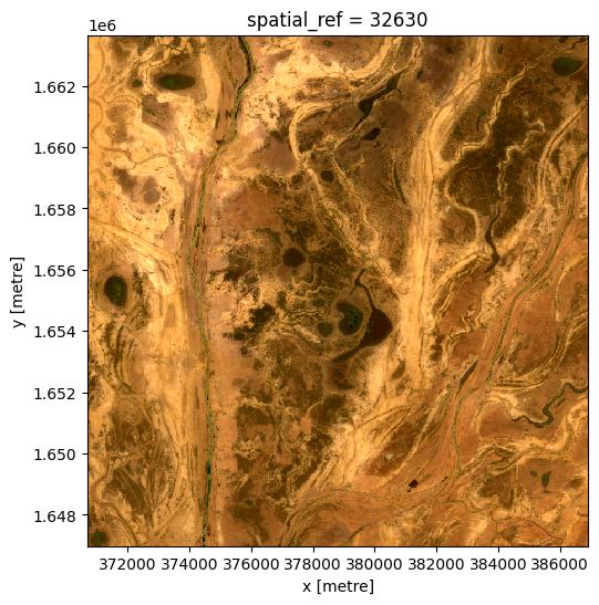
L’image composite après l’événement, du 03/06/2019 :

ds_after = da_after.to_dataset(dim='variable').drop_dims('variable')

rgb(ds_after, bands=['red', 'green', 'blue'])

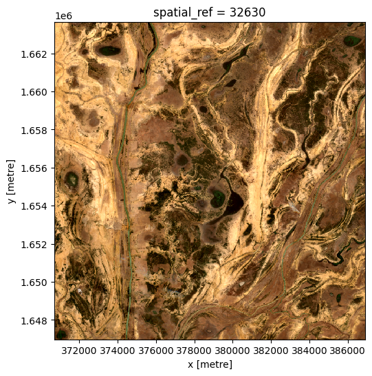
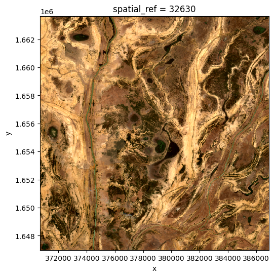
Composite du temps le plus proche

Parfois, nous souhaitons simplement obtenir les données disponibles les plus proches d’un moment précis. Ce composite prendra des valeurs antérieures ou postérieures à l’heure spécifiée pour trouver l’observation la plus proche.

da_nearest = nearest(da, dim='time', target='2019-06-03')

ds_nearest = da_nearest.to_dataset(dim='variable').drop_dims('variable')

rgb(ds_nearest, bands=['red', 'green', 'blue'])

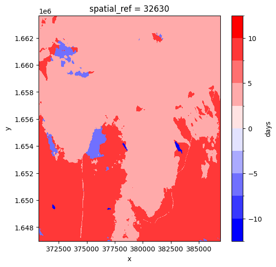
En regardant le « temps » pour chaque pixel, nous pouvons voir si le pixel a été pris avant ou après l’heure cible.

target_datetime = da_nearest.time.dtype.type('2019-06-03')

# calculate different in times and convert to number of days
num_days_different = (da_nearest.time.min(dim='variable') - target_datetime).dt.days

num_days_different.plot(cmap='bwr', levels=11, figsize=(6,6));

---

Informations Complémentaires

Licence : Le code de ce carnet est sous licence Apache, version 2.0 <https://www.apache.org/licenses/LICENSE-2.0>. Les données de Digital Earth Africa sont sous licence Creative Commons par attribution 4.0 <https://creativecommons.org/licenses/by/4.0/>.

Contact : Si vous avez besoin d’aide, veuillez poster une question sur le canal Slack Open Data Cube <http://slack.opendatacube.org/>`__ ou sur le GIS Stack Exchange en utilisant la balise open-data-cube (vous pouvez consulter les questions posées précédemment ici). Si vous souhaitez signaler un problème avec ce bloc-notes, vous pouvez en déposer un sur Github.

Version de Datacube compatible :

print(datacube.__version__)

1.8.15

Dernier test :

from datetime import datetime
datetime.today().strftime('%Y-%m-%d')

'2023-08-14'