Exécuter des analyses sur plusieurs polygones
Produits utilisés : s2_l2a
Mots-clés : analyse spatiale ; polygones, données utilisées ; sentinel-2, paquet python ; GeoPandas, index de bande ; NDVI
Aperçu
De nombreux utilisateurs ont besoin d’effectuer des analyses sur leurs propres domaines d’intérêt. Un cas d’utilisation courant consiste à exécuter la même analyse sur plusieurs polygones dans un fichier vectoriel (par exemple, ESRI Shapefile ou GeoJSON). Ce bloc-notes montrera comment utiliser un fichier vectoriel et Open Data Cube pour extraire des données satellite de Digital Earth Africa afin de faire correspondre les géométries de polygones individuels.
Description
Si nous avons un fichier vectoriel contenant plusieurs polygones, nous pouvons utiliser le package Python geopandas pour l’ouvrir en tant que GeoDataFrame. Nous pouvons ensuite parcourir chaque géométrie et extraire les données satellite correspondant à l’étendue de chaque géométrie. Une analyse plus approfondie peut ensuite être effectuée sur chaque xarray.Dataset résultant.
Dans ce bloc-notes, nous montrons comment récupérer des données pour chaque polygone et effectuer une analyse. L’exemple d’analyse dans ce bloc-notes consiste à charger et à tracer l’indice de végétation par différence normalisée (NDVI). Cette opération s’effectue selon les étapes suivantes :
Ouvrez le fichier de polygones en utilisant « geopandas ».
Parcourez le GeoDataFrame généré en extrayant les données satellite du cube de données ouvert de DE Africa.
Calculez le NDVI comme exemple d’analyse sur l’une des séries temporelles satellites extraites.
Tracez le NDVI pour l’étendue du polygone.
Commencer
Pour exécuter cette analyse, exécutez toutes les cellules du bloc-notes, en commençant par la cellule « Charger les packages ».
Charger des paquets
Veuillez noter l’utilisation du package « datacube.utils » « geometry » : ceci est important pour enregistrer le système de référence de coordonnées du fichier de formes entrant dans un format que la requête Digital Earth Africa peut comprendre.
[1]:
%matplotlib inline

import datacube
import matplotlib.pyplot as plt
import geopandas as gpd
from odc.geo.geom import Geometry
from odc.geo.crs import CRS

from deafrica_tools.datahandling import load_ard
from deafrica_tools.bandindices import calculate_indices
from deafrica_tools.plotting import rgb, map_shapefile
from deafrica_tools.spatial import xr_rasterize
from deafrica_tools.classification import HiddenPrints
Se connecter au datacube
Connectez-vous à la base de données Datacube pour activer le chargement des données de Digital Earth Australia.
[2]:
dc = datacube.Datacube(app='Analyse_multiple_polygons')
Paramètres d’analyse
time_range: saisissez une plage horaire pour votre requête, par exemple :('2019-01', '2019-12')si vous souhaitez des données pour toute l’année 2019vector_file: chemin d’accès à un fichier vectoriel (ESRI Shapefile ou GeoJSON) contenant des polygones à charger. Pour cet exemple, nous avons fourni un fichier Shapefile de démonstrationattribute_col: une colonne dans le fichier vectoriel utilisée pour étiqueter les jeux de données de sortiexarraycontenant des images satellite. Chaque ligne de cette colonne doit avoir un identifiant uniqueproducts: une liste de noms de produits à charger à partir du datacube, par exemple['ls8_c2l2', 'ls7_c2l2']. Dans cet exemple, nous utiliserons uniquement les données Sentinel-2,['s2_l2a']« mesures » : une liste de noms de bandes à charger à partir du produit satellite, par exemple « [“rouge”, “vert”] »
résolution: la résolution spatiale des données satellite chargées dans les directions « x » et « y » en mètres. Pour cet exemple Sentinel-2, nous avons sélectionné « (-20, 20) »output_crs: Le système de référence de coordonnées/projection cartographique dans lequel charger les données, par exemple « EPSG:6933 » pour charger les données dans une projection à surface égale pour l’Afrique
[3]:
time_range = ('2019-04', '2019-07')

vector_file = '../Supplementary_data/Analyse_multiple_polygons/multiple_polygons.shp'
attribute_col = 'id'

products = ['s2_l2a']
measurements = ['red', 'green', 'blue', 'nir']
resolution = (-20, 20)
output_crs = 'EPSG:6933'
Regardez la structure du fichier vectoriel
Importez le fichier et examinez sa structure afin de comprendre ce que nous parcourons. Le fichier contient trois polygones :
Nous mettrons également à jour la colonne « id » pour attribuer à chaque polygone un identifiant unique. Celui-ci sera utilisé pour identifier les données satellite correspondant au polygone dans le dictionnaire des résultats
[4]:
#read shapefile
gdf = gpd.read_file(vector_file)

# add an ID column
gdf['id']=range(0, len(gdf))

#print gdf
gdf.head()
[4]:
| id | class | geometry | |
|---|---|---|---|
| 0 | 0 | 0 | POLYGON ((-0.55603 7.66642, -0.52764 7.67401, ... |
| 1 | 1 | 0 | POLYGON ((-0.53018 7.64633, -0.49693 7.65515, ... |
| 2 | 2 | 0 | POLYGON ((-0.566 7.62164, -0.54007 7.6283, -0.... |
Nous pouvons ensuite tracer le « geopandas.GeoDataFrame » en utilisant la fonction « map_shapefile » pour nous assurer qu’il couvre la zone d’intérêt qui nous intéresse :
[5]:
map_shapefile(gdf, attribute=attribute_col)
Créer un objet de requête Datacube
Nous créons ensuite un dictionnaire qui contiendra les paramètres qui seront utilisés pour charger les données du datacube Digital Earth Africa :
Remarque : nous n’incluons pas ici les paramètres de requête spatiale habituels « x » et « y », car ils seront extraits directement de chacun de nos objets polygonaux vectoriels.
[6]:
query = {'time': time_range,
         'measurements': measurements,
         'resolution': resolution,
         'output_crs': output_crs,
         }

query
[6]:
{'time': ('2019-04', '2019-07'),
 'measurements': ['red', 'green', 'blue', 'nir'],
 'resolution': (-20, 20),
 'output_crs': 'EPSG:6933'}
Chargement des données satellite
Ici, nous allons parcourir chaque ligne de « geopandas.GeoDataFrame » et charger les données satellite. Les résultats seront ajoutés à un objet dictionnaire que nous pourrons ensuite indexer pour analyser chaque ensemble de données.
[7]:
# Dictionary to save results
results = {}

# A progress indicator
i = 0

# Loop through polygons in geodataframe and extract satellite data
for index, row in gdf.iterrows():

    print(" Feature {:02}/{:02}\r".format(i + 1, len(gdf)),
                  end='')

    # Get the geometry
    geom = Geometry(row.geometry.__geo_interface__, CRS(f'EPSG:{gdf.crs.to_epsg()}'))

    # Update dc query with geometry
    query.update({'geopolygon': geom})

    # Load landsat (hide print statements)
    with HiddenPrints():
        ds = load_ard(dc=dc,
                          products=products,
                          min_gooddata=0.75,
                          group_by='solar_day',
                          **query)

    # Generate a polygon mask to keep only data within the polygon
    with HiddenPrints():
        mask = xr_rasterize(gdf.iloc[[index]], ds)

    # Mask dataset to set pixels outside the polygon to `NaN`
    ds = ds.where(mask)

    # Append results to a dictionary using the attribute
    # column as an key
    results.update({str(row[attribute_col]) : ds})

    # Update counter
    i += 1
Feature 01/03
/opt/venv/lib/python3.12/site-packages/rasterio/warp.py:387: NotGeoreferencedWarning: Dataset has no geotransform, gcps, or rpcs. The identity matrix will be returned.
  dest = _reproject(
Feature 03/03
Analyse plus approfondie
Notre dictionnaire « résultats » contiendra des objets « xarray » étiquetés par les valeurs « attribute_col » uniques que nous avons spécifiées dans la section « Paramètres d’analyse » :
[8]:
results
[8]:
{'0': <xarray.Dataset> Size: 2MB
 Dimensions:      (time: 4, y: 192, x: 178)
 Coordinates:
   * time         (time) datetime64[ns] 32B 2019-05-02T10:39:04 ... 2019-06-26...
   * y            (y) float64 2kB 9.762e+05 9.761e+05 ... 9.724e+05 9.723e+05
   * x            (x) float64 1kB -5.365e+04 -5.363e+04 ... -5.013e+04 -5.011e+04
     spatial_ref  int32 4B 6933
 Data variables:
     red          (time, y, x) float32 547kB nan nan nan nan ... nan nan nan nan
     green        (time, y, x) float32 547kB nan nan nan nan ... nan nan nan nan
     blue         (time, y, x) float32 547kB nan nan nan nan ... nan nan nan nan
     nir          (time, y, x) float32 547kB nan nan nan nan ... nan nan nan nan
 Attributes:
     crs:           EPSG:6933
     grid_mapping:  spatial_ref,
 '1': <xarray.Dataset> Size: 3MB
 Dimensions:      (time: 6, y: 169, x: 178)
 Coordinates:
   * time         (time) datetime64[ns] 48B 2019-04-17T10:38:59 ... 2019-06-26...
   * y            (y) float64 1kB 9.738e+05 9.738e+05 ... 9.704e+05 9.704e+05
   * x            (x) float64 1kB -5.115e+04 -5.113e+04 ... -4.763e+04 -4.761e+04
     spatial_ref  int32 4B 6933
 Data variables:
     red          (time, y, x) float32 722kB nan nan nan nan ... nan nan nan nan
     green        (time, y, x) float32 722kB nan nan nan nan ... nan nan nan nan
     blue         (time, y, x) float32 722kB nan nan nan nan ... nan nan nan nan
     nir          (time, y, x) float32 722kB nan nan nan nan ... nan nan nan nan
 Attributes:
     crs:           EPSG:6933
     grid_mapping:  spatial_ref,
 '2': <xarray.Dataset> Size: 3MB
 Dimensions:      (time: 5, y: 189, x: 166)
 Coordinates:
   * time         (time) datetime64[ns] 40B 2019-04-12T10:39:01 ... 2019-06-26...
   * y            (y) float64 2kB 9.704e+05 9.704e+05 ... 9.666e+05 9.666e+05
   * x            (x) float64 1kB -5.461e+04 -5.459e+04 ... -5.133e+04 -5.131e+04
     spatial_ref  int32 4B 6933
 Data variables:
     red          (time, y, x) float32 627kB nan nan nan nan ... nan nan nan nan
     green        (time, y, x) float32 627kB nan nan nan nan ... nan nan nan nan
     blue         (time, y, x) float32 627kB nan nan nan nan ... nan nan nan nan
     nir          (time, y, x) float32 627kB nan nan nan nan ... nan nan nan nan
 Attributes:
     crs:           EPSG:6933
     grid_mapping:  spatial_ref}
Saisissez l’une de ces valeurs ci-dessous pour indexer notre dictionnaire et effectuer des analyses plus approfondies sur la série temporelle des satellites pour ce polygone.
[9]:
key = '2'
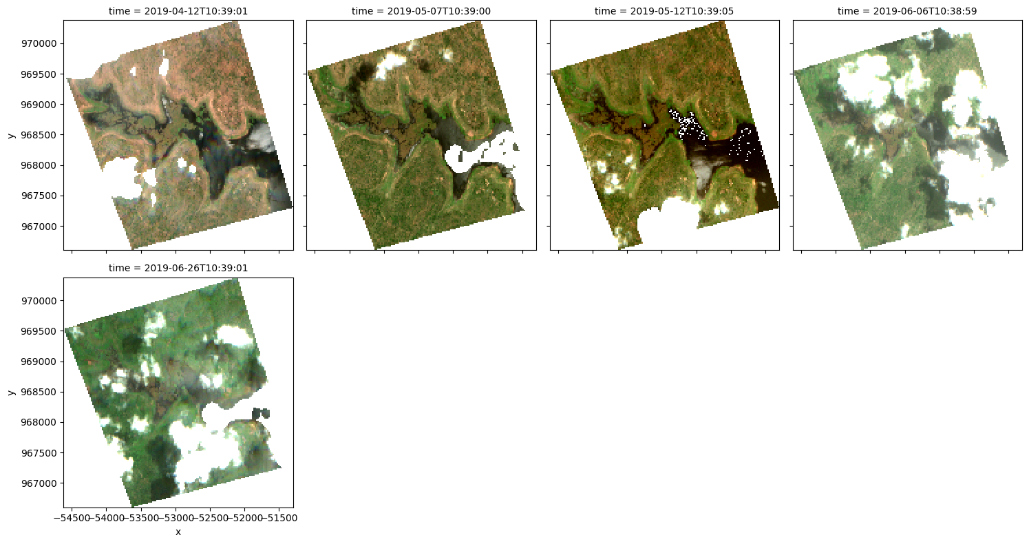
Tracer une image RVB
Nous pouvons maintenant utiliser la fonction « dea_plotting.rgb » pour tracer nos données chargées sous forme de tracé RVB à trois bandes :
[10]:
rgb(results[key], col='time', size=4)
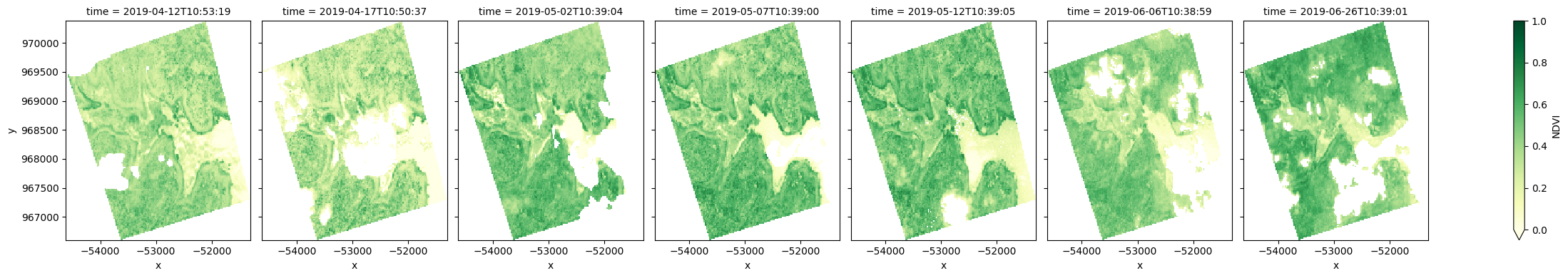
Calculer le NDVI et tracer
Nous pouvons également appliquer des analyses aux données chargées pour chacun de nos polygones. Par exemple, nous pouvons calculer l’indice de végétation par différence normalisée (NDVI) pour identifier les zones de végétation en croissance.
Remarque : le NDVI peut être calculé à l’aide de la fonction calculate_indices, importée depuis deafrica_tools.bandindices. Ici, nous utilisons
satellite_mission='s2'puisque nous travaillons avec les données Sentinel-2.
[11]:
# Calculate band index
ndvi = calculate_indices(results[key], index='NDVI', satellite_mission='s2')

# Plot NDVI for each polygon for the time query
ndvi.NDVI.plot(col='time', cmap='YlGn', vmin=0.0, vmax=1, figsize=(25, 4))
plt.show()
Informations Complémentaires
Licence : Le code de ce carnet est sous licence Apache, version 2.0 <https://www.apache.org/licenses/LICENSE-2.0>. Les données de Digital Earth Africa sont sous licence Creative Commons par attribution 4.0 <https://creativecommons.org/licenses/by/4.0/>.
Contact : Si vous avez besoin d’aide, veuillez poster une question sur le canal Slack Open Data Cube <http://slack.opendatacube.org/>`__ ou sur le GIS Stack Exchange en utilisant la balise open-data-cube (vous pouvez consulter les questions posées précédemment ici). Si vous souhaitez signaler un problème avec ce bloc-notes, vous pouvez en déposer un sur Github.
Version de Datacube compatible :
[12]:
print(datacube.__version__)
1.8.20
Dernier test :
[13]:
from datetime import datetime
datetime.today().strftime('%Y-%m-%d')
[13]:
'2025-01-15'