Combinaison de données satellitaires et de modélisation des marées à l’aide d’OTPS
Mots-clés données utilisées; landsat 5, données utilisées; landsat 7, données utilisées; landsat 8, marée; modélisation, intertidal, dask
Aperçu
Les marées océaniques sont des phénomènes de montée et de descente périodiques de l’océan provoqués par l’attraction gravitationnelle de la lune et du soleil et par la rotation de la terre. Les marées dans les zones côtières peuvent grandement influencer la façon dont ces environnements apparaissent sur les images satellite, car les niveaux d’eau varient jusqu’à 12 mètres. Pour pouvoir étudier les processus environnementaux le long du littoral africain, il est essentiel d’obtenir des données sur les conditions de marée au moment exact où chaque image satellite a été acquise.
Description
This notebook demonstrates how to combine remotely sensed imagery with information about ocean tides using functions from the eo-tides Python package, allowing us to analyse satellite imagery by tide heights and tidal stage (e.g. low, high, ebb, flow). These functions use the global ocean tide models to calculate the height (relative to mean sea level) and stage of the tide at the exact moment each satellite image was acquired.
Le cahier montre comment :
Charger un exemple de série chronologique de données satellitaires
Use the
tag_tidefunction fromeo-tides packageto model tide heights for each satellite observationUtiliser les données sur la hauteur des marées pour produire des composites médians de la côte à marée basse et haute
Calculer les données de phase de marée montante ou descendante pour déterminer si les niveaux d’eau montaient ou descendaient dans chaque observation satellite
Utilisez la fonction « tidal_stats » pour évaluer les éventuels biais dans les conditions de marée observées par un satellite
Commencer
Pour exécuter cette analyse, exécutez toutes les cellules du bloc-notes, en commençant par la cellule « Charger les packages ».
Charger des paquets
Installation Requirement
This notebook requires pyTMD version 2.2.9.
Please install it before running the imports:
```bash pip install pyTMD==2.2.9
[1]:
# pip install pyTMD==2.2.9
[2]:
import datacube
import xarray as xr
import geopandas as gpd
from odc.geo.geom import Geometry

from deafrica_tools.plotting import rgb, display_map
from deafrica_tools.datahandling import load_ard, mostcommon_crs
from eo_tides import tag_tides
from eo_tides.stats import tide_stats
from deafrica_tools.dask import create_local_dask_cluster
from deafrica_tools.areaofinterest import define_area
Configurer un cluster Dask
Dask peut être utilisé pour mieux gérer l’utilisation de la mémoire et effectuer l’analyse en parallèle. Pour une introduction à l’utilisation de Dask avec Digital Earth Africa, consultez le Dask notebook.
Remarque : nous vous recommandons d’ouvrir la fenêtre de traitement Dask pour afficher les différents calculs en cours d’exécution ; pour ce faire, consultez la section Tableau de bord Dask en Afrique de l’Ouest du Dask notebook.
Pour utiliser Dask, configurez le cluster de calcul local à l’aide de la cellule ci-dessous.
[3]:
create_local_dask_cluster()
Client
Client-de8ffd76-3319-11f1-86e0-66c27c7d89dc
| Connection method: Cluster object | Cluster type: distributed.LocalCluster |
| Dashboard: /user/mpho.sadiki@digitalearthafrica.org/proxy/36481/status |
Cluster Info
LocalCluster
516ebbfa
| Dashboard: /user/mpho.sadiki@digitalearthafrica.org/proxy/36481/status | Workers: 1 |
| Total threads: 4 | Total memory: 26.21 GiB |
| Status: running | Using processes: True |
Scheduler Info
Scheduler
Scheduler-c90d878d-9295-4cac-94b2-2a956be2d937
| Comm: tcp://127.0.0.1:35979 | Workers: 0 |
| Dashboard: /user/mpho.sadiki@digitalearthafrica.org/proxy/36481/status | Total threads: 0 |
| Started: Just now | Total memory: 0 B |
Workers
Worker: 0
| Comm: tcp://127.0.0.1:43187 | Total threads: 4 |
| Dashboard: /user/mpho.sadiki@digitalearthafrica.org/proxy/36327/status | Memory: 26.21 GiB |
| Nanny: tcp://127.0.0.1:44161 | |
| Local directory: /tmp/dask-scratch-space/worker-hmwwam_o | |
Se connecter au datacube
[4]:
dc = datacube.Datacube(app="Tidal_modelling")
Configurer la requête de données
Nous commençons par configurer une requête pour définir la zone, la période et les autres paramètres requis pour le chargement des données. Dans cet exemple, nous allons charger 30 ans de données Landsat 5, 7 et 8 pour l’estuaire de la rivière Geba dans le sud de la Guinée-Bissau. Nous chargeons les bandes « rouge », « verte », « bleue » afin de pouvoir représenter les données sous forme d’images en couleurs réelles.
Remarque : le paramètre « dask_chunks » nous permet d’utiliser Dask pour charger les données de manière différée plutôt que de les charger directement en mémoire <https://examples.dask.org/xarray.html>, car la méthode de chargement standard peut prendre beaucoup de temps et nécessiter beaucoup de mémoire. Le chargement différé peut être une approche très utile lorsque vous devez charger de grandes quantités de données sans faire planter votre analyse. Dans les applications côtières, il nous permet de charger (en utilisant soit « .compute() » soit en traçant nos données) uniquement un petit sous-ensemble d’observations de l’ensemble de notre série chronologique (par exemple, uniquement les observations de marée basse ou haute) sans avoir à charger l’ensemble des données en mémoire au préalable, ce qui peut réduire considérablement les temps de traitement.
Définir l’emplacement
Pour définir la zone d’intérêt, deux méthodes sont disponibles :
En spécifiant la latitude, la longitude et la zone tampon. Cette méthode nécessite que vous saisissiez la latitude centrale, la longitude centrale et la valeur de la zone tampon en degrés carrés autour du point central que vous souhaitez analyser. Par exemple, « lat = 10,338 », « lon = -1,055 » et « buffer = 0,1 » sélectionneront une zone avec un rayon de 0,1 degré carré autour du point avec les coordonnées (10,338, -1,055).
By uploading a polygon as a
GeoJSON or Esri Shapefile. If you choose this option, you will need to upload the geojson or ESRI shapefile into the Sandbox using Upload Files button in the top left corner of the Jupyter Notebook interface. ESRI shapefiles must be uploaded with all the related files
 (.cpg, .dbf, .shp, .shx). Once uploaded, you can use the shapefile or geojson to define the area of interest. Remember to update the code to call the file you have uploaded.
Pour utiliser l’une de ces méthodes, vous pouvez décommenter la ligne de code concernée et commenter l’autre. Pour commenter une ligne, ajoutez le symbole "#" avant le code que vous souhaitez commenter. Par défaut, la première option qui définit l’emplacement à l’aide de la latitude, de la longitude et du tampon est utilisée.
[5]:
# Define the location
# Method 1: Specify the latitude, longitude, and buffer
aoi = define_area(lat=11.689, lon=-15.674, buffer=0.15)

# Method 2: Use a polygon as a GeoJSON or Esri Shapefile.
# aoi = define_area(vector_path='aoi.shp')

# Create a geopolygon and geodataframe of the area of interest
geopolygon = Geometry(aoi["features"][0]["geometry"], crs="epsg:4326")
geopolygon_gdf = gpd.GeoDataFrame(geometry=[geopolygon], crs=geopolygon.crs)

# Get the latitude and longitude range of the geopolygon
lat_range = (geopolygon_gdf.total_bounds[1], geopolygon_gdf.total_bounds[3])
lon_range = (geopolygon_gdf.total_bounds[0], geopolygon_gdf.total_bounds[2])

# Create a reusable query
query = {
    "x": lon_range,
    "y": lat_range,
    "time": ("1988-01-01", "2018-12-31"),
    "measurements": ["red", "green", "blue"],
    "resolution": (-30, 30),
    "dask_chunks": {},
}
Nous pouvons prévisualiser la zone pour laquelle nous allons charger des données :
[6]:
display_map(x=query["x"], y=query["y"])
[6]:
Charger des séries chronologiques de satellites
Pour obtenir des données satellite à analyser, nous utilisons la fonction « load_ard » pour importer une série chronologique d’observations Landsat 5, 7 et 8 sous forme de « xarray.Dataset ». Les données d’entrée n’ont pas besoin de provenir de Landsat : toute imagerie de télédétection avec horodatage et coordonnées spatiales fournit suffisamment de données pour exécuter le modèle de marée.
[7]:
# Identify the most common projection system in the input query
output_crs = mostcommon_crs(dc=dc, product="ls8_sr", query=query)

# Load available data from all three Landsat satellites
ds = load_ard(
    dc=dc,
    products=["ls5_sr", "ls7_sr", "ls8_sr"],
    output_crs=output_crs,
    align=(15, 15),
    ls7_slc_off=False,
    group_by="solar_day",
    **query
)

# Print output data
print(ds)
Using pixel quality parameters for USGS Collection 2
Finding datasets
    ls5_sr
    ls7_sr
    Ignoring SLC-off observations for ls7
    ls8_sr
Applying pixel quality/cloud mask
Re-scaling Landsat C2 data
Returning 227 time steps as a dask array
<xarray.Dataset> Size: 3GB
Dimensions:      (time: 227, y: 1109, x: 1093)
Coordinates:
  * time         (time) datetime64[ns] 2kB 1988-07-17T10:52:47.658038 ... 201...
  * y            (y) float64 9kB 1.309e+06 1.309e+06 ... 1.276e+06 1.276e+06
  * x            (x) float64 9kB 4.102e+05 4.102e+05 ... 4.429e+05 4.429e+05
    spatial_ref  int32 4B 32628
Data variables:
    red          (time, y, x) float32 1GB dask.array<chunksize=(1, 1109, 1093), meta=np.ndarray>
    green        (time, y, x) float32 1GB dask.array<chunksize=(1, 1109, 1093), meta=np.ndarray>
    blue         (time, y, x) float32 1GB dask.array<chunksize=(1, 1109, 1093), meta=np.ndarray>
Attributes:
    crs:           EPSG:32628
    grid_mapping:  spatial_ref
/opt/venv/lib/python3.12/site-packages/deafrica_tools/datahandling.py:565: FutureWarning: In a future version of xarray the default value for compat will change from compat='no_conflicts' to compat='override'. This is likely to lead to different results when combining overlapping variables with the same name. To opt in to new defaults and get rid of these warnings now use `set_options(use_new_combine_kwarg_defaults=True) or set compat explicitly.
  ds = xr.merge([ds_data, ds_masks])
Modéliser les hauteurs de marée pour chaque observation
We can now pass our satellite dataset ds to the tag_tides function to model a tide for each timestep in our dataset.
The tag_tides function uses the time and date of acquisition and the geographic centroid of each satellite observation as inputs for the selected tide model (EOT20 by default). It returns an xarray.DataArray called tide_height, with a modelled tide for every timestep in our satellite dataset:
[8]:
# # Model tide heights
model_dir = "/var/share/tide_models"

tides_da = tag_tides(
    data=ds,
    directory=model_dir,
)

# Print modelled tides
tides_da
Setting tide modelling location from dataset centroid: -15.67, 11.69
Modelling tides with EOT20
[8]:
<xarray.DataArray 'tide_height' (time: 227)> Size: 908B
array([ 0.8592769 , -0.18536592, -0.24930622, -0.21912642,  1.3536943 ,
        1.5856296 , -0.36671248, -1.162862  , -0.84991807,  0.78121537,
        1.2990576 ,  0.5875723 , -0.5906921 , -1.198272  , -0.87473166,
       -0.23873524, -0.46583444,  0.8389599 ,  1.2147173 , -0.90109295,
        2.2094488 , -0.10366018, -0.7232631 ,  0.93119794,  0.09051751,
       -1.5260075 ,  0.4858677 , -1.0699933 , -0.9408271 , -0.7329113 ,
        2.3638723 ,  1.5525019 ,  0.1859477 , -1.1284522 ,  0.02373447,
        1.9752105 ,  1.4451119 ,  0.08928777, -1.1222141 , -0.9019982 ,
       -1.0450093 ,  0.79601216,  2.3718722 ,  1.4501921 , -0.06832927,
       -1.0044726 , -1.0839821 ,  0.17514926,  1.235538  ,  1.4246706 ,
        0.99165756, -1.0692114 , -0.80042666,  0.8843542 ,  1.5233799 ,
        2.4851034 ,  0.8361768 , -0.30938658, -1.2930602 , -1.010503  ,
       -0.8662913 ,  1.3671592 ,  1.7509861 , -0.29216802, -0.8316837 ,
        0.6845504 ,  0.9089041 ,  1.5951457 ,  2.4264863 ,  1.636322  ,
        1.1844784 ,  0.6951644 , -0.5465059 , -1.1753923 , -1.0261688 ,
       -1.1895244 , -0.65899706,  0.6656056 ,  1.5154617 ,  1.7234896 ,
        1.0035887 , -0.26266134, -0.8812882 , -1.418292  , -0.77705395,
        0.09498855,  0.34845093,  1.3668454 ,  2.103673  ,  1.6849209 ,
        1.6869351 , -0.23761284, -0.5975377 , -0.8819262 , -1.2235104 ,
       -0.49499667,  0.59162694, -0.21275352,  0.59459233,  1.6347721 ,
...
       -0.9089948 , -0.27688542, -0.162714  ,  1.245498  ,  1.928993  ,
        1.8759419 ,  2.3370724 ,  1.5809414 ,  0.30614835, -0.11390533,
       -0.92469454, -1.5192188 , -0.9430964 , -0.40575445, -0.19064783,
        1.0995171 ,  1.6986959 ,  1.7050391 ,  2.1494768 ,  1.3949219 ,
        0.20653185, -0.14812092, -1.0164082 , -1.4779083 , -0.7888232 ,
       -0.31432354,  1.4256083 ,  1.9217592 ,  2.3725417 ,  1.3677355 ,
        0.12567818, -0.16532955, -1.123294  , -1.5323508 , -0.8538998 ,
       -0.4728178 ,  0.01170299,  1.2474009 ,  1.7048676 ,  1.7812264 ,
        2.1977248 ,  1.234935  ,  0.09342687, -0.1761156 , -1.1653123 ,
       -1.4053906 , -0.6627003 ,  0.30462867,  1.5867989 ,  1.9666264 ,
        2.3179724 ,  1.1569254 , -0.02334541, -0.24811259, -1.2985601 ,
       -1.4740304 , -0.7577282 , -0.5203916 ,  0.24021955,  1.3851444 ,
        1.6893141 ,  1.8696413 ,  2.1551821 ,  1.0754136 ,  0.01313501,
       -0.23448984, -1.2910479 , -1.2690802 , -0.53377897,  0.5520059 ,
        1.7250115 ,  1.8446099 ,  2.008283  ,  2.1571045 ,  0.95168877,
       -0.13945593, -0.35539186, -1.4434679 , -1.3494217 , -0.66648966,
       -0.5192263 ,  0.45858455,  1.50598   ,  1.6530383 ,  1.971703  ,
        2.0207052 ,  0.925047  , -1.3809084 , -1.0875833 , -0.41610128,
        0.7656607 ,  1.8128856 ,  1.733615  ,  2.0340157 ,  1.9105709 ,
        0.7570475 , -0.20097291], dtype=float32)
Coordinates:
  * time        (time) datetime64[ns] 2kB 1988-07-17T10:52:47.658038 ... 2018...
tide_model <U5 20B 'EOT20'We can easily combine these modelled tides with our original satellite data for further analysis. The code below adds our modelled tides as a new tide_height variable under Data variables.
[9]:
ds["tide_height"] = tides_da
ds
[9]:
<xarray.Dataset> Size: 3GB
Dimensions:      (time: 227, y: 1109, x: 1093)
Coordinates:
  * time         (time) datetime64[ns] 2kB 1988-07-17T10:52:47.658038 ... 201...
  * y            (y) float64 9kB 1.309e+06 1.309e+06 ... 1.276e+06 1.276e+06
  * x            (x) float64 9kB 4.102e+05 4.102e+05 ... 4.429e+05 4.429e+05
    spatial_ref  int32 4B 32628
    tide_model   <U5 20B 'EOT20'
Data variables:
    red          (time, y, x) float32 1GB dask.array<chunksize=(1, 1109, 1093), meta=np.ndarray>
    green        (time, y, x) float32 1GB dask.array<chunksize=(1, 1109, 1093), meta=np.ndarray>
    blue         (time, y, x) float32 1GB dask.array<chunksize=(1, 1109, 1093), meta=np.ndarray>
    tide_height  (time) float32 908B 0.8593 -0.1854 -0.2493 ... 0.757 -0.201
Attributes:
    crs:           EPSG:32628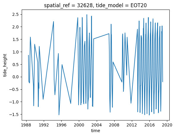
grid_mapping: spatial_refNous pouvons facilement représenter graphiquement cette nouvelle variable pour inspecter la plage de hauteurs de marée observées par les satellites dans notre série temporelle. Dans cet exemple, nos hauteurs de marée observées varient d’environ -1,0 à 1,0 m par rapport au niveau moyen de la mer :
[10]:
ds.tide_height.plot()
[10]:
[<matplotlib.lines.Line2D at 0x7f026370dd60>]
Exemple d’analyse de la hauteur des marées
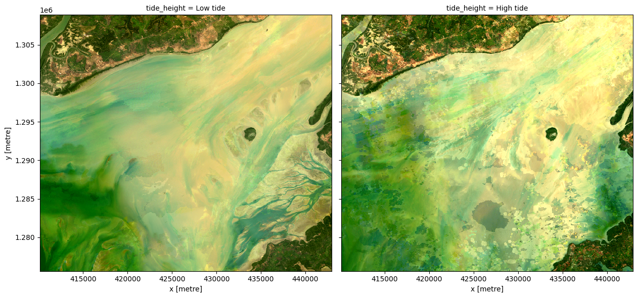
Pour démontrer comment les images marquées par les marées peuvent être utilisées pour produire des composites d’images de marée haute et basse, nous pouvons calculer les 5 % les plus bas et les 5 % les plus hauts des hauteurs de marée, et les utiliser pour filtrer nos observations. Nous pouvons ensuite combiner et tracer ces observations filtrées pour visualiser à quoi ressemble le paysage à marée basse et à marée haute :
Remarque : nous vous recommandons d’ouvrir la fenêtre de traitement Dask pour afficher les différents calculs en cours d’exécution ; pour ce faire, consultez la section Tableau de bord Dask en Afrique de l’Ouest du Dask notebook.
Remarque : une approche alternative pour combiner des observations dans un composite peut être obtenue en utilisant un géomédian, ce qui garantit que les relations entre les bandes restent cohérentes. Des informations supplémentaires sont fournies dans le bloc-notes « Génération de composites géomédians <Generating_geomedian_composites.ipynb> ».
[11]:
# Calculate the lowest and highest 5% of tides
lowest_5, highest_5 = ds.tide_height.quantile([0.05, 0.95]).values

# Filter our data to low and high tide observations
filtered_low = ds.where(ds.tide_height <= lowest_5, drop=True)
filtered_high = ds.where(ds.tide_height >= highest_5, drop=True)

# Take the simple median of each set of low and high tide observations to
# produce a composite (alternatively, observations could be combined
# using a geomedian to keep band relationships consistent)
median_low = filtered_low.median(dim="time", keep_attrs=True)
median_high = filtered_high.median(dim="time", keep_attrs=True)

# Combine low and high tide medians into a single dataset and give
# each layer a meaningful name
ds_highlow = xr.concat([median_low, median_high], dim="tide_height")
ds_highlow["tide_height"] = ["Low tide", "High tide"]

# Plot low and high tide medians side-by-side
rgb(ds_highlow, col="tide_height")
Modélisation des phases de marée montante et descendante
The tag_tides function also allows us to determine whether each satellite observation was taken while the tide was rising/incoming (flow tide) or falling/outgoing (ebb tide) by setting return_phases=True. This is achieved by comparing tide heights 15 minutes before and after the observed satellite observation.
Les données de flux et de reflux peuvent fournir des informations contextuelles précieuses pour l’interprétation des images satellite, en particulier dans les environnements de vasières ou de forêts de mangroves où l’eau peut rester dans le paysage pendant un temps considérable après le pic de marée.
[12]:
tides_da = tag_tides(
    data=ds,
    directory=model_dir,
    return_phases=True,
)

# Print modelled tides
tides_da
Setting tide modelling location from dataset centroid: -15.67, 11.69
Modelling tides with EOT20
Modelling tides with EOT20
[12]:
<xarray.Dataset> Size: 5kB
Dimensions:      (time: 227)
Coordinates:
  * time         (time) datetime64[ns] 2kB 1988-07-17T10:52:47.658038 ... 201...
    tide_model   <U5 20B 'EOT20'
Data variables:
    tide_height  (time) float32 908B 0.8593 -0.1854 -0.2493 ... 0.757 -0.201
tide_phase (time) object 2kB 'high-flow' 'low-flow' ... 'low-flow'Nous disposons désormais de données nous indiquant à la fois la hauteur de la marée et la phase de marée (« flux » ou « reflux ») pour chaque image satellite :
[13]:
tides_da[["time", "tide_height", "tide_phase"]].to_dataframe()
[13]:
| tide_height | tide_phase | tide_model | |
|---|---|---|---|
| time | |||
| 1988-07-17 10:52:47.658038 | 0.859277 | high-flow | EOT20 |
| 1988-08-18 10:52:49.179013 | -0.185366 | low-flow | EOT20 |
| 1988-10-05 10:52:43.680006 | -0.249306 | low-ebb | EOT20 |
| 1988-10-21 10:52:37.662000 | -0.219126 | low-ebb | EOT20 |
| 1988-12-08 10:52:31.815006 | 1.353694 | high-ebb | EOT20 |
| ... | ... | ... | ... |
| 2018-10-24 11:21:58.388427 | 1.733615 | high-ebb | EOT20 |
| 2018-11-09 11:22:01.151598 | 2.034016 | high-flow | EOT20 |
| 2018-11-25 11:22:00.936674 | 1.910571 | high-flow | EOT20 |
| 2018-12-11 11:21:57.773631 | 0.757047 | high-flow | EOT20 |
| 2018-12-27 11:21:57.806437 | -0.200973 | low-flow | EOT20 |
227 rows × 3 columns
Nous pourrions par exemple utiliser ces données pour filtrer nos observations afin de ne conserver que les observations en phase de reflux :
[14]:
tides_da.where(tides_da.tide_phase.str.contains("ebb"), drop=True)
[14]:
<xarray.Dataset> Size: 2kB
Dimensions:      (time: 108)
Coordinates:
  * time         (time) datetime64[ns] 864B 1988-10-05T10:52:43.680006 ... 20...
    tide_model   <U5 20B 'EOT20'
Data variables:
    tide_height  (time) float32 432B -0.2493 -0.2191 1.354 ... 1.813 1.734
tide_phase (time) object 864B 'low-ebb' 'low-ebb' ... 'high-ebb'Évaluation des hauteurs de marée observées par rapport à toutes les hauteurs de marée modélisées
Le comportement complexe des marées signifie qu’un capteur héliosynchrone comme Landsat « n’observe pas l’intégralité du cycle des marées à tous les endroits <https://www.sciencedirect.com/science/article/pii/S0272771418308783#sec3> ». Des biais dans la proportion de l’amplitude des marées observée par les satellites peuvent nous empêcher d’obtenir des données sur les zones du littoral exposées ou inondées aux extrémités de l’amplitude des marées. Cela peut risquer d’obtenir des informations trompeuses sur l’étendue réelle de la zone du littoral affectée par les marées et rendre difficile la comparaison équitable des images de marée haute ou basse dans différents endroits.
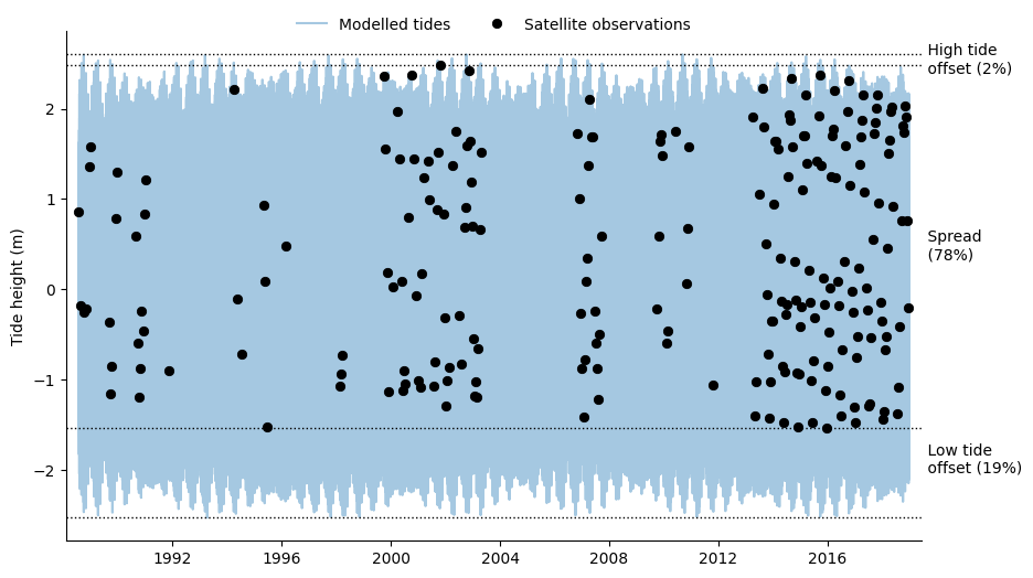
The tide_stats function can assist in evaluating how the range of tides observed by satellites compare to the full tidal range. It works by using the OTPS tidal model to model tide heights at a regular interval (every two hours by default) across the entire time period covered by the input satelliter timeseries dataset. This is then compared against the tide heights in observed by the satellite and used to calculate a range of statistics and a plot that summarises potential biases in the
data.
Remarque : pour une discussion plus détaillée de la question du biais de marée dans les observations par satellite héliosynchrones du littoral, reportez-vous à la section « Limitations et travaux futurs » dans Bishop-Taylor et al. 2018 <https://www.sciencedirect.com/science/article/pii/S0272771418308783#sec3>`__.
[15]:
out_stats = tide_stats(data=ds, directory=model_dir)
Using tide modelling location: -15.67, 11.69
Modelling tides with EOT20
Using tide modelling location: -15.67, 11.69
Modelling tides with EOT20


🌊 Modelled astronomical tide range: 5.13 m (-2.53 to 2.60 m).
🛰️ Observed tide range: 4.02 m (-1.53 to 2.49 m).

🟡 78% of the modelled astronomical tide range was observed at this location.
🟢 The highest 2% (0.12 m) of the tide range was never observed.
🟡 The lowest 19% (1.00 m) of the tide range was never observed.

🌊 Mean modelled astronomical tide height: 0.00 m.
🛰️ Mean observed tide height: 0.34 m.
⬆️ The mean observed tide height was 0.34 m higher than the mean modelled astronomical tide height.
The tide_stats function also outputs a pandas.Series object containing a set of statistics that compare the observed vs. full modelled tidal ranges. These statistics include:
mot: mean tide height observed by the satellite (metres)
mat: mean modelled astronomical tide height (metres)
hot: maximum tide height observed by the satellite (metres)
hat: maximum tide height from modelled astronomical tidal range (metres)
lot: minimum tide height observed by the satellite (metres)
lat: minimum tide height from modelled astronomical tidal range (metres)
otr: tidal range observed by the satellite (metres)
tr: modelled astronomical tide range (metres)
spread: proportion of the full modelled tidal range observed by the satellite
offset_low: proportion of the lowest tides never observed by the satellite
offset_high: proportion of the highest tides never observed by the satellite
y: latitude used for modelling tide heights
x: longitude used for modelling tide heights
[16]:
print(out_stats)
mot             0.344
mat             0.000
hot             2.485
hat             2.603
lot            -1.532
lat            -2.529
otr             4.017
tr              5.131
spread          0.783
offset_low      0.194
offset_high     0.023
x             -15.674
y              11.689
dtype: float32
Informations Complémentaires
Licence : Le code de ce carnet est sous licence Apache, version 2.0 <https://www.apache.org/licenses/LICENSE-2.0>. Les données de Digital Earth Africa sont sous licence Creative Commons par attribution 4.0 <https://creativecommons.org/licenses/by/4.0/>.
Contact : Si vous avez besoin d’aide, veuillez poster une question sur le canal Slack Open Data Cube <http://slack.opendatacube.org/>`__ ou sur le GIS Stack Exchange en utilisant la balise open-data-cube (vous pouvez consulter les questions posées précédemment ici). Si vous souhaitez signaler un problème avec ce bloc-notes, vous pouvez en déposer un sur Github.
Version de Datacube compatible :
[17]:
print(datacube.__version__)
1.9.13
Dernier test :
[18]:
from datetime import datetime

datetime.today().strftime("%Y-%m-%d")
[18]:
'2026-04-08'