Intégration de données externes à partir d’un fichier CSV
Produits utilisés : ls8_sr
Mots clés données utilisées ; landsat 8, données externes, méthodes de données ; interpolation, données utilisées ; csv, intertidal, coastal, water
Aperçu
Il est souvent utile de combiner des données externes (par exemple à partir d’un fichier CSV ou d’un autre ensemble de données) avec des données chargées à partir de Digital Earth Africa. Par exemple, nous pouvons vouloir combiner des données provenant d’un indicateur de marée ou d’un indicateur de rivière avec des données satellite pour déterminer les niveaux d’eau au moment exact où chaque observation satellite a été effectuée. Cela peut nous permettre de manipuler et d’extraire des données satellite et d’obtenir des informations supplémentaires à l’aide de données provenant de notre source externe.
Description
Cet exemple de bloc-notes charge une série chronologique de données de modélisation de marée externes à partir d’un fichier CSV et les combine avec des données satellite chargées à partir de Digital Earth Africa. Ce flux de travail peut être appliqué à n’importe quel ensemble de données de séries chronologiques externes (par exemple, jauges fluviales, jauges de marée, mesures de précipitations, etc.). Le bloc-notes montre comment :
Charger une série chronologique de données Landsat 8
Charger des données de séries chronologiques externes à partir d’un fichier CSV
Convertissez ces données en un « xarray.Dataset » et liez-les à chaque observation satellite en interpolant les valeurs à chaque pas de temps satellite
Ajoutez ces nouvelles données en tant que variable dans notre ensemble de données satellite et utilisez-les pour filtrer les images satellite en images de marée haute et basse
Montrez comment échanger les dimensions entre « time » et la nouvelle variable « tide_height »
Commencer
Pour exécuter cette analyse, exécutez toutes les cellules du bloc-notes, en commençant par la cellule « Charger les packages ».
Charger des paquets
[1]:
%matplotlib inline

import datacube
import pandas as pd
import geopandas as gpd
import matplotlib.pyplot as plt
from odc.geo.geom import Geometry

from deafrica_tools.datahandling import load_ard, mostcommon_crs
from deafrica_tools.areaofinterest import define_area

pd.plotting.register_matplotlib_converters()
Se connecter au datacube
[2]:
dc = datacube.Datacube(app='Integrating_external_data')
Chargement des données satellite
Nous chargeons d’abord trois années de données Landsat 8. Nous utiliserons la baie de Msasani en Tanzanie pour cette démonstration, car nous disposons d’un fichier CSV de données sur la hauteur des marées pour cet endroit que nous souhaitons combiner avec des données satellite. Nous chargeons une seule bande « nir » qui différencie clairement l’eau (valeurs basses) et la terre (valeurs élevées). Cela nous permettra de vérifier que nous pouvons utiliser des données de marée externes pour identifier les observations satellite de marée basse et de marée haute.
Pour définir la zone d’intérêt, deux méthodes sont disponibles :
En spécifiant la latitude, la longitude et la zone tampon. Cette méthode nécessite que vous saisissiez la latitude centrale, la longitude centrale et la valeur de la zone tampon en degrés carrés autour du point central que vous souhaitez analyser. Par exemple, « lat = 10,338 », « lon = -1,055 » et « buffer = 0,1 » sélectionneront une zone avec un rayon de 0,1 degré carré autour du point avec les coordonnées (10,338, -1,055).
By uploading a polygon as a
GeoJSON or Esri Shapefile. If you choose this option, you will need to upload the geojson or ESRI shapefile into the Sandbox using Upload Files button in the top left corner of the Jupyter Notebook interface. ESRI shapefiles must be uploaded with all the related files
 (.cpg, .dbf, .shp, .shx). Once uploaded, you can use the shapefile or geojson to define the area of interest. Remember to update the code to call the file you have uploaded.
Pour utiliser l’une de ces méthodes, vous pouvez décommenter la ligne de code concernée et commenter l’autre. Pour commenter une ligne, ajoutez le symbole "#" avant le code que vous souhaitez commenter. Par défaut, la première option qui définit l’emplacement à l’aide de la latitude, de la longitude et du tampon est utilisée.
[3]:
# Set the area of interest
# Method 1: Specify the latitude, longitude, and buffer
aoi = define_area(lat=-6.745, lon=39.261, buffer=0.06)

# Method 2: Use a polygon as a GeoJSON or Esri Shapefile.
# aoi = define_area(vector_path='aoi.shp')

#Create a geopolygon and geodataframe of the area of interest
geopolygon = Geometry(aoi["features"][0]["geometry"], crs="epsg:4326")
geopolygon_gdf = gpd.GeoDataFrame(geometry=[geopolygon], crs=geopolygon.crs)

# Get the latitude and longitude range of the geopolygon
lat_range = (geopolygon_gdf.total_bounds[1], geopolygon_gdf.total_bounds[3])
lon_range = (geopolygon_gdf.total_bounds[0], geopolygon_gdf.total_bounds[2])


# Create a reusable query
query = {
    'x': lon_range,
    'y': lat_range,
    'time': ('2015-01-01', '2017-12-31'),
    'measurements': ['nir'],
    'resolution': (-30, 30)
}

# Identify the most common projection system in the input query
output_crs = mostcommon_crs(dc=dc, product='ls8_sr', query=query)

# Load Landsat 8 data
ds = load_ard(dc=dc,
              products=['ls8_sr'],
              output_crs=output_crs,
              align=(15, 15),
              group_by='solar_day',
              **query)

print(ds)
Using pixel quality parameters for USGS Collection 2
Finding datasets
    ls8_sr
Applying pixel quality/cloud mask
Re-scaling Landsat C2 data
Loading 65 time steps
<xarray.Dataset> Size: 51MB
Dimensions:      (time: 65, y: 443, x: 443)
Coordinates:
  * time         (time) datetime64[ns] 520B 2015-01-07T07:32:04.385652 ... 20...
  * y            (y) float64 4kB -7.389e+05 -7.39e+05 ... -7.522e+05 -7.522e+05
  * x            (x) float64 4kB 5.222e+05 5.222e+05 ... 5.354e+05 5.355e+05
    spatial_ref  int32 4B 32637
Data variables:
    nir          (time, y, x) float32 51MB nan nan nan ... 0.006718 0.006443
Attributes:
    crs:           epsg:32637
    grid_mapping:  spatial_ref
Intégration de données externes
Charger dans un fichier CSV des données externes avec horodatage
Dans le code ci-dessous, nous visons à prendre un fichier CSV de données externes (dans ce cas, les hauteurs de marée toutes les demi-heures pour un emplacement dans la baie de Msasani, en Tanzanie pour une période de cinq ans entre 2014 et 2018 générées à l’aide du modèle de marée OTPS TPXO8 <https://www.tpxo.net/global/tpxo8-atlas>`__), et à relier ces données à notre série chronologique de données satellite.
Nous pouvons charger les données de hauteur de marée existantes en utilisant le module « pandas » que nous avons importé précédemment. Les données ont une colonne de valeurs « time », que nous définirons comme colonne d’index (à peu près équivalente à une « dimension » dans « xarray »).
[4]:
tide_data = pd.read_csv('../Supplementary_data/Integrating_external_data/msasani_bay_-6.749102_39.261819_2014-2018_tides.csv',
                          parse_dates=['time'],
                          index_col='time')

tide_data.head()
[4]:
| tide_height | |
|---|---|
| time | |
| 2014-01-01 00:00:00 | 1.798 |
| 2014-01-01 00:30:00 | 1.885 |
| 2014-01-01 01:00:00 | 1.867 |
| 2014-01-01 01:30:00 | 1.743 |
| 2014-01-01 02:00:00 | 1.521 |
Lier des données externes à des données satellite
Maintenant que nous disposons des données sur la hauteur de la marée, nous devons estimer la hauteur de la marée pour chacune de nos images satellite. Nous pouvons le faire en interpolant entre les points de données dont nous disposons (mesures horaires) pour obtenir une estimation de la hauteur de la marée au moment exact où chaque image satellite a été prise.
Le code ci-dessous génère un « xarray.Dataset » avec le même nombre de pas de temps que les données satellite d’origine. L’ensemble de données possède une seule variable « tide_height » qui donne la hauteur de marée estimée pour chaque observation :
[5]:
# First, we convert the data to an xarray dataset so we can analyse it
# in the same way as our satellite data
tide_data_xr = tide_data.to_xarray()

# We want to convert our hourly tide heights to estimates of exactly how
# high the tide was at the time that each satellite image was taken. To
# do this, we can use `.interp` to 'interpolate' a tide height for each
# satellite timestamp:
satellite_tideheights = tide_data_xr.interp(time=ds.time)

# Print the output xarray object
print(satellite_tideheights)
<xarray.Dataset> Size: 1kB
Dimensions:      (time: 65)
Coordinates:
  * time         (time) datetime64[ns] 520B 2015-01-07T07:32:04.385652 ... 20...
    spatial_ref  int32 4B 32637
Data variables:
    tide_height  (time) float64 520B -1.401 -1.382 -0.7692 ... -0.2992 -0.3579
Nous avons maintenant nos hauteurs de marée au format « xarray » qui correspondent à nos données satellite. Nous pouvons les ajouter à notre ensemble de données satellite en tant que nouvelle variable :
[6]:
# We then want to put these values back into the Landsat dataset so
# that each image has an estimated tide height:
ds['tide_height'] = satellite_tideheights.tide_height
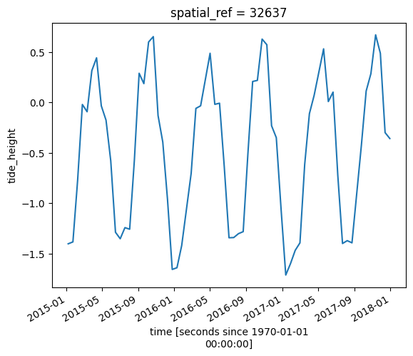
Nous pouvons désormais tracer les hauteurs de marée pour nos données satellite :
[7]:
# Plot the resulting tide heights for each Landsat image:
ds.tide_height.plot()
plt.show()
Filtrage par données externes
Maintenant que nous avons une nouvelle variable « tide_height » dans notre ensemble de données, nous pouvons utiliser les méthodes d’indexation « xarray » pour manipuler nos données en utilisant les hauteurs de marée (par exemple, filtrer par marée pour sélectionner des images de marée basse ou haute) :
[8]:
# Select a subset of low tide images (tide less than -1.0 m)
low_tide_ds = ds.sel(time = ds.tide_height < -1.0)

# Select a subset of high tide images (tide greater than 0.1 m)
high_tide_ds = ds.sel(time = ds.tide_height > 0.1)
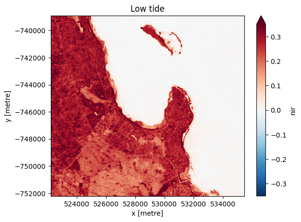
Nous pouvons tracer la médiane des images filtrées pour la marée basse et la marée haute afin d’examiner la différence entre elles. Prendre la médiane nous permet de visualiser une image sans nuages.
Pour les images de marée basse :
[9]:
# Compute the median of all low tide images to produce a single cloud free image.
low_tide_composite = low_tide_ds.median(dim='time', skipna=True, keep_attrs=False)

# Plot the median low tide image
low_tide_composite.nir.plot(robust=True)
plt.title('Low tide')
plt.show()
et pour les images de marée haute :
[10]:
# Compute the median of all high tide images to produce a single cloud free image.
high_tide_composite = high_tide_ds.median(dim='time', skipna=True, keep_attrs=False)

# Plot the median high tide image
high_tide_composite.nir.plot(robust=True)
plt.title('High tide')
plt.show()
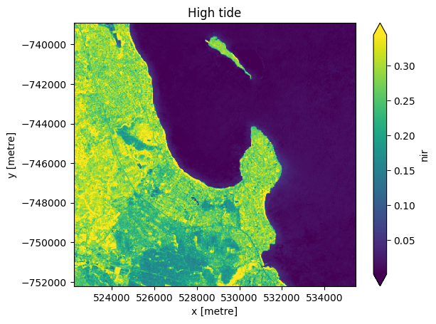
Notez que de nombreuses zones de marée basse sur l’image de marée basse (bleu-vert) apparaissent désormais inondées par l’eau (bleu foncé/violet) sur l’image de marée haute.
Échange de dimensions en fonction de données externes
Par défaut, « xarray » utilise « time » comme l’une des dimensions principales de l’ensemble de données (en plus de « x » et « y »). Maintenant que nous avons une nouvelle variable « tide_height », nous pouvons la modifier pour qu’elle devienne une dimension réelle dans l’ensemble de données à la place de « time ». Cela permet des opérations supplémentaires plus avancées, telles que le calcul de statistiques glissantes ou l’agrégation par « tide_heights ».
Dans l’exemple ci-dessous, vous pouvez voir que l’ensemble de données comporte désormais trois dimensions (tide_height, x et y). La dimension time n’est plus une dimension de l’ensemble de données.
[11]:
print(ds.swap_dims({'time': 'tide_height'}))
<xarray.Dataset> Size: 51MB
Dimensions:      (tide_height: 65, y: 443, x: 443)
Coordinates:
    time         (tide_height) datetime64[ns] 520B 2015-01-07T07:32:04.385652...
  * y            (y) float64 4kB -7.389e+05 -7.39e+05 ... -7.522e+05 -7.522e+05
  * x            (x) float64 4kB 5.222e+05 5.222e+05 ... 5.354e+05 5.355e+05
    spatial_ref  int32 4B 32637
  * tide_height  (tide_height) float64 520B -1.401 -1.382 ... -0.2992 -0.3579
Data variables:
    nir          (tide_height, y, x) float32 51MB nan nan ... 0.006718 0.006443
Attributes:
    crs:           epsg:32637
    grid_mapping:  spatial_ref
Informations Complémentaires
Licence : Le code de ce carnet est sous licence Apache, version 2.0 <https://www.apache.org/licenses/LICENSE-2.0>. Les données de Digital Earth Africa sont sous licence Creative Commons par attribution 4.0 <https://creativecommons.org/licenses/by/4.0/>.
Contact : Si vous avez besoin d’aide, veuillez poster une question sur le canal Slack Open Data Cube <http://slack.opendatacube.org/>`__ ou sur le GIS Stack Exchange en utilisant la balise open-data-cube (vous pouvez consulter les questions posées précédemment ici). Si vous souhaitez signaler un problème avec ce bloc-notes, vous pouvez en déposer un sur Github.
Version de Datacube compatible :
[12]:
print(datacube.__version__)
1.8.20
Dernier test :
[13]:
from datetime import datetime
datetime.today().strftime('%Y-%m-%d')
[13]:
'2025-01-15'