Extraction des courbes de niveau
Mots clés données utilisées ; sentinel-2, données utilisées ; SRTM, méthodes de données ; extraction de contour, analyse ; traitement d’image, indice de bande ; NDWI
Aperçu
L’extraction de contours <https://en.wikipedia.org/wiki/Contour_line> est une méthode fondamentale de traitement d’images utilisée pour détecter et extraire les limites des entités spatiales. Alors que l’extraction de contours a traditionnellement été utilisée pour cartographier avec précision des lignes d’élévation donnée à partir de modèles numériques d’élévation (MNE), les contours peuvent également être extraits de toute autre source de données basée sur un tableau. Cela peut être utilisé pour prendre en charge les applications de télédétection où la position d’une limite précise doit être cartographiée de manière cohérente au fil du temps, comme l’extraction de limites de lignes de flottaison dynamiques à partir de données d’indice de différence normalisée de l’eau (NDWI) dérivées de satellites.
Description
Ce bloc-notes montre comment utiliser la fonction « subpixel_contours » basée sur les outils de « skimage.measure.find_contours » pour :
Extraire une ou plusieurs courbes de niveau à partir d’un seul modèle numérique d’élévation (MNE) bidimensionnel et les exporter sous forme de fichier de formes
Inclure éventuellement des attributs personnalisés dans les entités de contour extraites
Chargez un ensemble de données satellite multidimensionnelles à partir de Digital Earth Africa et extrayez une valeur de contour unique de manière cohérente au fil du temps le long d’une dimension spécifiée
Filtrer les contours obtenus pour supprimer les petites caractéristiques bruyantes
Commencer
Pour exécuter cette analyse, exécutez toutes les cellules du bloc-notes, en commençant par la cellule « Charger les packages ».
Charger des paquets
[1]:
%matplotlib inline

import datacube
import numpy as np
import pandas as pd
import xarray as xr
import warnings
import matplotlib as mpl
import matplotlib.pyplot as plt
from odc.ui import with_ui_cbk
import geopandas as gpd
from odc.geo.geom import Geometry

from deafrica_tools.spatial import subpixel_contours
from deafrica_tools.bandindices import calculate_indices
from deafrica_tools.areaofinterest import define_area
Se connecter au datacube
[2]:
dc = datacube.Datacube(app='Contour_extraction')
Paramètres d’analyse
La cellule suivante définit les paramètres qui définissent la zone d’intérêt et la durée de l’analyse. Les paramètres sont
« lat » : la latitude centrale à analyser (par exemple « 6,502 »).
« lon » : la longitude centrale à analyser (par exemple « -1,409 »).
« buffer » : le nombre de degrés carrés à charger autour de la latitude et de la longitude centrales. Pour des temps de chargement raisonnables, définissez cette valeur sur « 0,1 » ou moins.
Pour définir la zone d’intérêt, deux méthodes sont disponibles :
En spécifiant la latitude, la longitude et la zone tampon. Cette méthode nécessite que vous saisissiez la latitude centrale, la longitude centrale et la valeur de la zone tampon en degrés carrés autour du point central que vous souhaitez analyser. Par exemple, « lat = 10,338 », « lon = -1,055 » et « buffer = 0,1 » sélectionneront une zone avec un rayon de 0,1 degré carré autour du point avec les coordonnées (10,338, -1,055).
By uploading a polygon as a
GeoJSON or Esri Shapefile. If you choose this option, you will need to upload the geojson or ESRI shapefile into the Sandbox using Upload Files button in the top left corner of the Jupyter Notebook interface. ESRI shapefiles must be uploaded with all the related files
 (.cpg, .dbf, .shp, .shx). Once uploaded, you can use the shapefile or geojson to define the area of interest. Remember to update the code to call the file you have uploaded.
Pour utiliser l’une de ces méthodes, vous pouvez décommenter la ligne de code concernée et commenter l’autre. Pour commenter une ligne, ajoutez le symbole "#" avant le code que vous souhaitez commenter. Par défaut, la première option qui définit l’emplacement à l’aide de la latitude, de la longitude et du tampon est utilisée.
Si vous exécutez le bloc-notes pour la première fois, conservez les paramètres par défaut ci-dessous. Cela montrera comment fonctionne l’analyse et fournira des résultats significatifs. L’exemple porte sur le lac Bosomtwe, l’un des plus grands lacs d’Afrique de l’Ouest.
Pour exécuter le bloc-notes pour une zone différente, assurez-vous que les données Sentinel-2 sont disponibles pour la zone choisie à l’aide de DEAfrica Explorer. Utilisez le menu déroulant pour vérifier la couverture de s2_l2a.
[3]:
# # buffer will define the upper and lower boundary from the central point
# buffer = 0.2

# Method 1: Specify the latitude, longitude, and buffer
aoi = define_area(lat=-3.064, lon=37.359, buffer=0.2)

# Method 2: Use a polygon as a GeoJSON or Esri Shapefile.
#aoi = define_area(vector_path='aoi.shp')

#Create a geopolygon and geodataframe of the area of interest
geopolygon = Geometry(aoi["features"][0]["geometry"], crs="epsg:4326")
geopolygon_gdf = gpd.GeoDataFrame(geometry=[geopolygon], crs=geopolygon.crs)

# Get the latitude and longitude range of the geopolygon
lat_range = (geopolygon_gdf.total_bounds[1], geopolygon_gdf.total_bounds[3])
lon_range = (geopolygon_gdf.total_bounds[0], geopolygon_gdf.total_bounds[2])
Données d’élévation de charge
Pour démontrer l’extraction de contours, nous devons d’abord obtenir un ensemble de données d’élévation. Le datacube de DE Africa contient un modèle numérique d’élévation (DEM) de la mission de topographie radar de la navette spatiale (SRTM), nous pouvons donc charger les données d’élévation directement à partir du datacube à l’aide de « dc.load ». Dans cet exemple, les coordonnées ci-dessus correspondent à une région autour du mont Kilimandjaro.
[4]:
# Create a reusable query
query = {
    'x': lon_range,
    'y': lat_range,
    'output_crs': 'EPSG:6933',
    'resolution': (-30, 30)
}

#load data
elevation_array = dc.load(product ='dem_srtm', **query)
elevation_array
[4]:
<xarray.Dataset> Size: 4MB
Dimensions:      (time: 1, y: 1699, x: 1287)
Coordinates:
  * time         (time) datetime64[ns] 8B 2000-01-01T12:00:00
  * y            (y) float64 14kB -3.652e+05 -3.653e+05 ... -4.162e+05
  * x            (x) float64 10kB 3.585e+06 3.585e+06 ... 3.624e+06 3.624e+06
    spatial_ref  int32 4B 6933
Data variables:
    elevation    (time, y, x) int16 4MB 1890 1894 1894 1892 ... 1641 1643 1644
Attributes:
    crs:           EPSG:6933
grid_mapping: spatial_refLe « xarray » renvoyé contient une seule entrée dans la dimension temporelle. Pour faciliter l’utilisation du « xarray », nous pouvons appliquer la méthode « .squeeze() », qui supprime toutes les dimensions où il n’y a qu’une seule entrée (« time » dans ce cas).
[5]:
#Use the squeeze method to remove any 1 dimensional value from the dataset. eg time = 1
elevation_array = elevation_array.squeeze()

#convert to an dataArray rather an Dataset
elevation_array = elevation_array['elevation']
elevation_array
[5]:
<xarray.DataArray 'elevation' (y: 1699, x: 1287)> Size: 4MB
array([[1890, 1894, 1894, ..., 1452, 1452, 1449],
       [1891, 1894, 1894, ..., 1454, 1452, 1449],
       [1891, 1894, 1894, ..., 1454, 1452, 1449],
       ...,
       [1137, 1137, 1136, ..., 1643, 1643, 1643],
       [1137, 1137, 1136, ..., 1643, 1643, 1643],
       [1134, 1130, 1131, ..., 1641, 1643, 1644]], dtype=int16)
Coordinates:
    time         datetime64[ns] 8B 2000-01-01T12:00:00
  * y            (y) float64 14kB -3.652e+05 -3.653e+05 ... -4.162e+05
  * x            (x) float64 10kB 3.585e+06 3.585e+06 ... 3.624e+06 3.624e+06
    spatial_ref  int32 4B 6933
Attributes:
    units:         metre
    nodata:        -32768.0
    crs:           EPSG:6933
grid_mapping: spatial_refTracer les données chargées
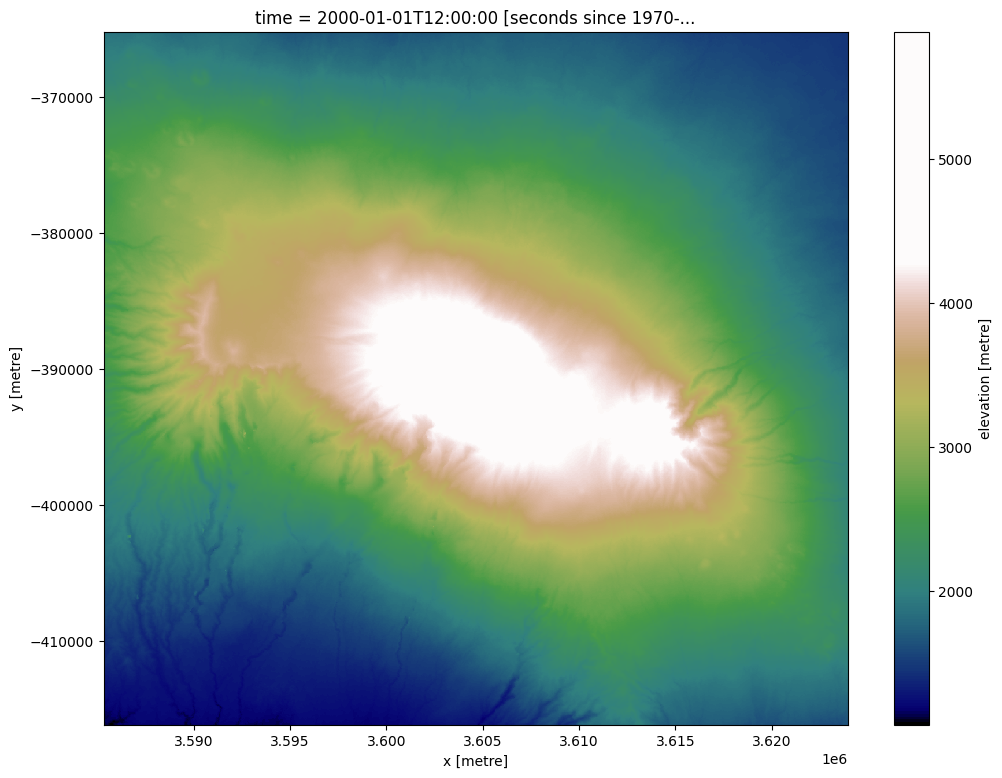
Nous pouvons tracer les données d’élévation pour une région autour du mont Kilimandjaro à l’aide d’une carte couleur personnalisée du terrain :
[6]:
# Create a custom colourmap for the DEM
colors_terrain = plt.cm.gist_earth(np.linspace(0.0, 1.5, 100))
cmap_terrain = mpl.colors.LinearSegmentedColormap.from_list('terrain', colors_terrain)

# Plot a subset of the elevation data
elevation_array.plot(size=9, cmap=cmap_terrain)
[6]:
<matplotlib.collections.QuadMesh at 0x7f2bf7960980>
Extraction de contours en mode « tableau unique, valeurs z multiples »
La fonction « deafrica_spatialtools.subpixel_contours » utilise « skimage.measure.find_contours » pour extraire les courbes de niveau d’un tableau. Il peut s’agir d’un ensemble de données d’élévation comme les données importées ci-dessus, ou de tout autre tableau bidimensionnel ou multidimensionnel. Nous pouvons extraire les contours du tableau d’élévation importé ci-dessus en fournissant une seule valeur z (par exemple, l’élévation) ou une liste de valeurs z.
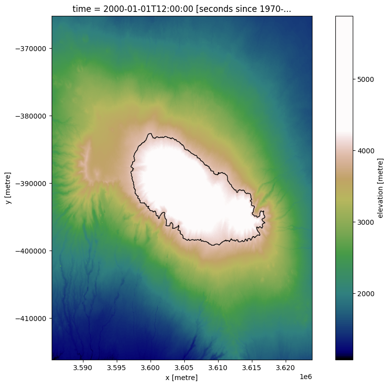
Extraction d’un seul contour
Ici, nous extrayons un seul contour d’élévation de 4000 m :
[7]:
# Extract contours
contours_gdf = subpixel_contours(da=elevation_array,
                                 z_values=[4000])

# Print output
contours_gdf
Operating in multiple z-value, single array mode
[7]:
| z_value | geometry | |
|---|---|---|
| 0 | 4000 | MULTILINESTRING ((3609135 -399258.75, 3609105 ... |
Cela renvoie un « geopandas.GeoDataFrame » contenant une seule entité de ligne de contour avec la valeur z (c’est-à-dire l’altitude) donnée dans un champ de fichier de formes nommé « z_value ». Nous pouvons tracer le contour extrait sur le DEM :
[8]:
elevation_array.plot(size=9, cmap=cmap_terrain)
contours_gdf.plot(ax=plt.gca(), linewidth=1.0, color='black')
[8]:
<Axes: title={'center': 'time = 2000-01-01T12:00:00 [seconds since 1970-...'}, xlabel='x [metre]', ylabel='y [metre]'>
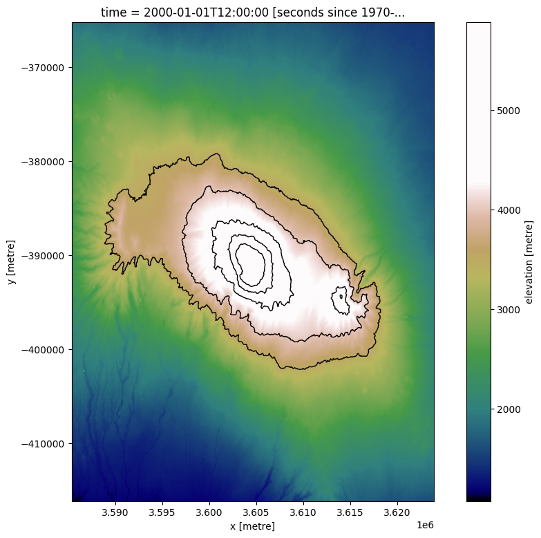
Extraction de plusieurs contours
Nous pouvons facilement importer plusieurs contours à partir d’un seul tableau en fournissant une liste de valeurs z à extraire. La fonction extraira ensuite un contour pour chaque valeur dans « z_values », en ignorant toute élévation de contour qui ne se trouve pas dans le tableau.
[9]:
# List of elevations to extract
z_values = [3500, 4000, 4500, 5000, 5500]

# Extract contours
contours_gdf = subpixel_contours(da=elevation_array,
                                 z_values=z_values)

# Plot extracted contours over the DEM
elevation_array.plot(size=9, cmap=cmap_terrain)
contours_gdf.plot(ax=plt.gca(), linewidth=1.0, color='black')
Operating in multiple z-value, single array mode
[9]:
<Axes: title={'center': 'time = 2000-01-01T12:00:00 [seconds since 1970-...'}, xlabel='x [metre]', ylabel='y [metre]'>
Attributs de shapefile personnalisés
Par défaut, le fichier de formes inclut un seul champ d’attribut « z_value » avec une entité par valeur d’entrée dans « z_values ». Nous pouvons à la place transmettre des attributs personnalisés au fichier de formes de sortie à l’aide du paramètre « attribute_df ». Par exemple, nous pourrions vouloir une colonne personnalisée appelée « elev_km » avec des hauteurs en kilomètres (km) au lieu de mètres (m), et une colonne « location » indiquant l’emplacement, le mont Kilamanjaro (KLJ).
Nous pouvons y parvenir en créant d’abord un « pandas.DataFrame » avec des noms de colonnes indiquant le nom de l’attribut que nous voulons inclure avec nos entités de contour, et une ligne de valeurs pour chaque nombre dans « z_values » :
[10]:
# Elevation values to extract in metres
z_values = [2000, 3000, 5500]

# Set up attribute dataframe (one row per elevation value above)
attribute_df = pd.DataFrame({'elev_km': [2, 3, 5.5],
                             'location': ['KLJ1', 'KLJ2', 'KLJ3']})

# Print output
attribute_df.head()
[10]:
| elev_km | location | |
|---|---|---|
| 0 | 2.0 | KLJ1 |
| 1 | 3.0 | KLJ2 |
| 2 | 5.5 | KLJ3 |
Nous pouvons maintenant extraire les contours, et les entités de contour résultantes incluront les attributs que nous avons créés ci-dessus :
[11]:
# Extract contours with custom attribute fields:
contours_gdf = subpixel_contours(da=elevation_array,
                                 z_values=z_values,
                                 attribute_df=attribute_df)

# Print output
contours_gdf.head()
Operating in multiple z-value, single array mode
[11]:
| z_value | elev_km | location | geometry | |
|---|---|---|---|---|
| 0 | 2000 | 2.0 | KLJ1 | MULTILINESTRING ((3585345 -367545, 3585375 -36... |
| 1 | 3000 | 3.0 | KLJ2 | MULTILINESTRING ((3609975 -405387, 3609945 -40... |
| 2 | 5500 | 5.5 | KLJ3 | MULTILINESTRING ((3604575 -393350, 3604545 -39... |
Exportation des contours vers un fichier
Pour exporter les contours obtenus dans un fichier, utilisez le paramètre « output_path ». La fonction prend en charge deux formats de fichier de sortie :
GéoJSON (.geojson)
Fichier de formes (.shp)
[12]:
subpixel_contours(da=elevation_array,
                  z_values=z_values,
                  output_path='output_contours.geojson')
Operating in multiple z-value, single array mode
Writing contours to output_contours.geojson
[12]:
| z_value | geometry | |
|---|---|---|
| 0 | 2000 | MULTILINESTRING ((3585345 -367545, 3585375 -36... |
| 1 | 3000 | MULTILINESTRING ((3609975 -405387, 3609945 -40... |
| 2 | 5500 | MULTILINESTRING ((3604575 -393350, 3604545 -39... |
Courbes de niveau à partir d’ensembles de données non altimétriques en mode « valeur z unique, tableaux multiples »
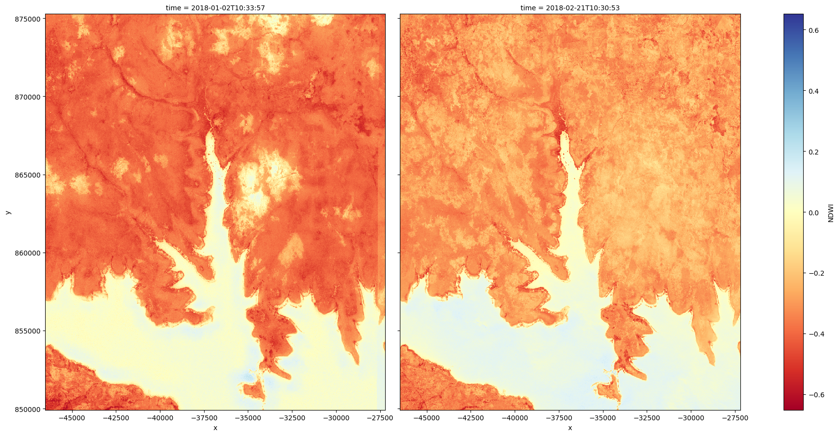
En plus d’extraire plusieurs contours d’un seul tableau bidimensionnel, subpixel_contours vous permet également d’extraire une seule valeur z de chaque tableau le long d’une dimension spécifiée dans un tableau multidimensionnel. Cela peut être utile pour comparer les changements du paysage au fil du temps. Le tableau multidimensionnel d’entrée n’a pas besoin d’être constitué de données d’élévation : les contours peuvent être extraits de n’importe quel type de données.
Par exemple, nous pouvons utiliser la fonction pour extraire la limite entre la terre et l’eau (pour une analyse plus approfondie utilisant l’extraction de contours pour surveiller l’érosion côtière, voir ce bloc-notes). Tout d’abord, nous allons charger une série chronologique d’images Sentinel-2 et calculer un simple indice d’eau par différence normalisée (NDWI) sur deux images. Cet indice aura des valeurs élevées là où un pixel est susceptible d’être en eau libre (par exemple, NDWI > 0, coloré en bleu ci-dessous) :
[13]:
# Set up a datacube query to load data for
# first provide a new location (Lake Volta in Ghana)
lat, lon = 6.777, -0.382
buffer = 0.1

#set-up a query
query = {
        'x': (lon-buffer, lon+buffer),
        'y': (lat+buffer, lat-buffer),
         'time': ('2018-01-01', '2018-02-25'),
         'measurements': ['nir_1', 'green'],
         'output_crs': 'EPSG:6933',
         'resolution': (-20, 20)}

# Load Sentinel 2 data
s2_ds = dc.load(product='s2_l2a',
                group_by='solar_day',
                progress_cbk=with_ui_cbk(),
                **query)
s2_ds
[13]:
<xarray.Dataset> Size: 54MB
Dimensions:      (time: 11, y: 1268, x: 966)
Coordinates:
  * time         (time) datetime64[ns] 88B 2018-01-02T10:33:57 ... 2018-02-21...
  * y            (y) float64 10kB 8.753e+05 8.752e+05 ... 8.5e+05 8.499e+05
  * x            (x) float64 8kB -4.651e+04 -4.649e+04 ... -2.723e+04 -2.721e+04
    spatial_ref  int32 4B 6933
Data variables:
    nir_1        (time, y, x) uint16 27MB 2120 2216 2202 2188 ... 720 716 753
    green        (time, y, x) uint16 27MB 1062 1090 1082 1068 ... 906 904 916
Attributes:
    crs:           EPSG:6933
grid_mapping: spatial_refCalculer le NDWI sur la première et la dernière image de l’ensemble de données
[14]:
s2_ds = calculate_indices(s2_ds.isel(time=[0, -1]),
                          index='NDWI',
                          satellite_mission='s2'
                         )


# Plot the two images side by size
s2_ds.NDWI.plot(col='time', cmap='RdYlBu', size=9)
[14]:
<xarray.plot.facetgrid.FacetGrid at 0x7f2c6927b500>
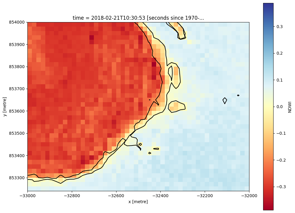
Nous pouvons maintenant identifier la limite terre-eau en extrayant le contour NDWI 0 pour chaque tableau de l’ensemble de données le long de la dimension « temps ». En traçant les lignes de contour résultantes pour une zone agrandie, nous pouvons alors commencer à comparer des phénomènes tels que les niveaux des lacs au fil du temps.
[15]:
# Extract the 0 NDWI contour from both timesteps in the NDWI data
contours_gdf = subpixel_contours(da=s2_ds.NDWI,
                                 z_values=0,
                                 crs=s2_ds.geobox.crs,
                                 dim='time')

# Plot contours over the top of array
s2_ds.NDWI.isel(time=-1).sel(x = slice(-33000, -32000),
                        y = slice(854000, 853250)).plot(size = 9, cmap = 'RdYlBu')

contours_gdf.plot(ax = plt.gca(), linewidth = 1.5, color = 'black')
Operating in single z-value, multiple arrays mode
[15]:
<Axes: title={'center': 'time = 2018-02-21T10:30:53 [seconds since 1970-...'}, xlabel='x [metre]', ylabel='y [metre]'>
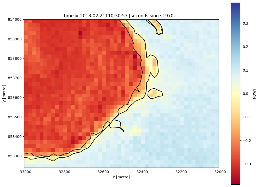
Abandonner les petits contours
Les contours produits par « subpixel_contours » peuvent inclure de nombreuses petites entités. Nous pouvons éventuellement choisir d’extraire uniquement les contours plus grands qu’un certain nombre de sommets à l’aide du paramètre « min_vertices ». Cela peut être utile pour se concentrer sur les grands contours et supprimer le bruit éventuel dans un ensemble de données. Ici, nous définissons « min_vertices=10 » pour ne conserver que les contours avec au moins 10 sommets. Observez la disparition du petit plan d’eau en bas à gauche de l’image :
[16]:
# Extract the 0 NDWI contour from both timesteps in the NDWI data
contours_gdf = subpixel_contours(da=s2_ds.NDWI,
                                 z_values=0,
                                 crs=s2_ds.geobox.crs,
                                 min_vertices=10)

# Plot contours over the top of array
# Plot contours over the top of array
s2_ds.NDWI.isel(time=-1).sel(x = slice(-33000, -32000),
                        y = slice(854000, 853250)).plot(size = 9, cmap = 'RdYlBu')

contours_gdf.plot(ax = plt.gca(), linewidth = 1.5, color = 'black')
Operating in single z-value, multiple arrays mode
[16]:
<Axes: title={'center': 'time = 2018-02-21T10:30:53 [seconds since 1970-...'}, xlabel='x [metre]', ylabel='y [metre]'>
Informations Complémentaires
Licence : Le code de ce carnet est sous licence Apache, version 2.0 <https://www.apache.org/licenses/LICENSE-2.0>. Les données de Digital Earth Africa sont sous licence Creative Commons par attribution 4.0 <https://creativecommons.org/licenses/by/4.0/>.
Contact : Si vous avez besoin d’aide, veuillez poster une question sur le canal Slack Open Data Cube <http://slack.opendatacube.org/>`__ ou sur le GIS Stack Exchange en utilisant la balise open-data-cube (vous pouvez consulter les questions posées précédemment ici). Si vous souhaitez signaler un problème avec ce bloc-notes, vous pouvez en déposer un sur Github.
Version de Datacube compatible :
[17]:
print(datacube.__version__)
1.8.20
Dernier test :
[18]:
from datetime import datetime
datetime.today().strftime('%Y-%m-%d')
[18]:
'2025-01-15'