Extracting contour lines
Keywords data used; sentinel-2, data used; SRTM, data methods; contour extraction, analysis; image processing, band index; NDWI
Background
Contour extraction is a fundamental image processing method used to detect and extract the boundaries of spatial features. While contour extraction has traditionally been used to precisely map lines of given elevation from digital elevation models (DEMs), contours can also be extracted from any other array-based data source. This can be used to support remote sensing applications where the position of a precise boundary needs to be mapped consistently over time, such as extracting dynamic waterline boundaries from satellite-derived Normalized Difference Water Index (NDWI) data.
Description
This notebook demonstrates how to use the subpixel_contours function based on tools from skimage.measure.find_contours to:
Extract one or multiple contour lines from a single two-dimensional digital elevation model (DEM) and export these as a shapefile
Optionally include custom attributes in the extracted contour features
Load in a multi-dimensional satellite dataset from Digital Earth Africa, and extract a single contour value consistently through time along a specified dimension
Filter the resulting contours to remove small noisy features
Getting started
To run this analysis, run all the cells in the notebook, starting with the “Load packages” cell.
Load packages
[1]:
%matplotlib inline

import datacube
import numpy as np
import pandas as pd
import xarray as xr
import warnings
import matplotlib as mpl
import matplotlib.pyplot as plt
from odc.ui import with_ui_cbk
import geopandas as gpd
from odc.geo.geom import Geometry

from deafrica_tools.spatial import subpixel_contours
from deafrica_tools.bandindices import calculate_indices
from deafrica_tools.areaofinterest import define_area
Connect to the datacube
[2]:
dc = datacube.Datacube(app='Contour_extraction')
Analysis parameters
The following cell sets the parameters, which define the area of interest and the length of time to conduct the analysis over. The parameters are
lat: The central latitude to analyse (e.g.6.502).lon: The central longitude to analyse (e.g.-1.409).buffer: The number of square degrees to load around the central latitude and longitude. For reasonable loading times, set this as0.1or lower.
To define the area of interest, there are two methods available:
By specifying the latitude, longitude, and buffer. This method requires you to input the central latitude, central longitude, and the buffer value in square degrees around the center point you want to analyze. For example,
lat = 10.338,lon = -1.055, andbuffer = 0.1will select an area with a radius of 0.1 square degrees around the point with coordinates (10.338, -1.055).By uploading a polygon as a
GeoJSON or Esri Shapefile. If you choose this option, you will need to upload the geojson or ESRI shapefile into the Sandbox using Upload Files button in the top left corner of the Jupyter Notebook interface. ESRI shapefiles must be uploaded with all the related files
 (.cpg, .dbf, .shp, .shx). Once uploaded, you can use the shapefile or geojson to define the area of interest. Remember to update the code to call the file you have uploaded.
To use one of these methods, you can uncomment the relevant line of code and comment out the other one. To comment out a line, add the "#" symbol before the code you want to comment out. By default, the first option which defines the location using latitude, longitude, and buffer is being used.
If running the notebook for the first time, keep the default settings below. This will demonstrate how the analysis works and provide meaningful results. The example covers Lake Bosomtwe, one of the largest lakes in Western Africa.
To run the notebook for a different area, make sure Sentinel-2 data is available for the chosen area using the DEAfrica Explorer. Use the drop-down menu to check coverage for s2_l2a.
[3]:
# # buffer will define the upper and lower boundary from the central point
# buffer = 0.2

# Method 1: Specify the latitude, longitude, and buffer
aoi = define_area(lat=-3.064, lon=37.359, buffer=0.2)

# Method 2: Use a polygon as a GeoJSON or Esri Shapefile.
#aoi = define_area(vector_path='aoi.shp')

#Create a geopolygon and geodataframe of the area of interest
geopolygon = Geometry(aoi["features"][0]["geometry"], crs="epsg:4326")
geopolygon_gdf = gpd.GeoDataFrame(geometry=[geopolygon], crs=geopolygon.crs)

# Get the latitude and longitude range of the geopolygon
lat_range = (geopolygon_gdf.total_bounds[1], geopolygon_gdf.total_bounds[3])
lon_range = (geopolygon_gdf.total_bounds[0], geopolygon_gdf.total_bounds[2])
Load elevation data
To demonstrate contour extraction, we first need to obtain an elevation dataset. DE Africa’s datacube contains a Digital Elevation Model (DEM) from the Shuttle Radar Topography Mission (SRTM), so we can load in elevation data directly from the datacube using dc.load. In this example, the coordinates above correpsond to a region around Mount Kilimanjaro.
[4]:
# Create a reusable query
query = {
    'x': lon_range,
    'y': lat_range,
    'output_crs': 'EPSG:6933',
    'resolution': (-30, 30)
}

#load data
elevation_array = dc.load(product ='dem_srtm', **query)
elevation_array
[4]:
<xarray.Dataset> Size: 4MB
Dimensions:      (time: 1, y: 1699, x: 1287)
Coordinates:
  * time         (time) datetime64[ns] 8B 2000-01-01T12:00:00
  * y            (y) float64 14kB -3.652e+05 -3.653e+05 ... -4.162e+05
  * x            (x) float64 10kB 3.585e+06 3.585e+06 ... 3.624e+06 3.624e+06
    spatial_ref  int32 4B 6933
Data variables:
    elevation    (time, y, x) int16 4MB 1890 1894 1894 1892 ... 1641 1643 1644
Attributes:
    crs:           EPSG:6933
grid_mapping: spatial_refThe returned xarray has a single entry in the time dimension. To make the xarray easier to work with, we can apply the .squeeze() method, which remove any dimensions where there is only one entry (time in this case).
[5]:
#Use the squeeze method to remove any 1 dimensional value from the dataset. eg time = 1
elevation_array = elevation_array.squeeze()

#convert to an dataArray rather an Dataset
elevation_array = elevation_array['elevation']
elevation_array
[5]:
<xarray.DataArray 'elevation' (y: 1699, x: 1287)> Size: 4MB
array([[1890, 1894, 1894, ..., 1452, 1452, 1449],
       [1891, 1894, 1894, ..., 1454, 1452, 1449],
       [1891, 1894, 1894, ..., 1454, 1452, 1449],
       ...,
       [1137, 1137, 1136, ..., 1643, 1643, 1643],
       [1137, 1137, 1136, ..., 1643, 1643, 1643],
       [1134, 1130, 1131, ..., 1641, 1643, 1644]], dtype=int16)
Coordinates:
    time         datetime64[ns] 8B 2000-01-01T12:00:00
  * y            (y) float64 14kB -3.652e+05 -3.653e+05 ... -4.162e+05
  * x            (x) float64 10kB 3.585e+06 3.585e+06 ... 3.624e+06 3.624e+06
    spatial_ref  int32 4B 6933
Attributes:
    units:         metre
    nodata:        -32768.0
    crs:           EPSG:6933
grid_mapping: spatial_refPlot the loaded data
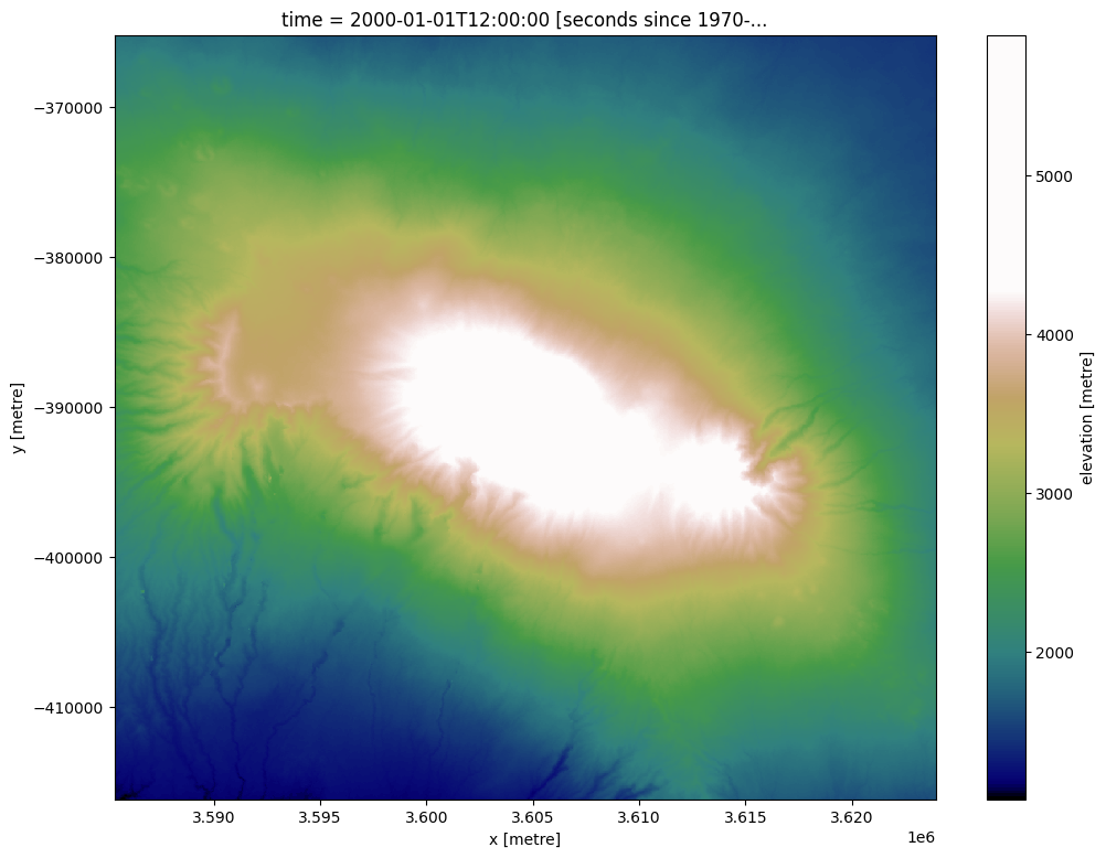
We can plot the elevation data for a region around Mount Kilimanjaro using a custom terrain-coloured colour map:
[6]:
# Create a custom colourmap for the DEM
colors_terrain = plt.cm.gist_earth(np.linspace(0.0, 1.5, 100))
cmap_terrain = mpl.colors.LinearSegmentedColormap.from_list('terrain', colors_terrain)

# Plot a subset of the elevation data
elevation_array.plot(size=9, cmap=cmap_terrain)
[6]:
<matplotlib.collections.QuadMesh at 0x7f2bf7960980>
Contour extraction in ‘single array, multiple z-values’ mode
The deafrica_spatialtools.subpixel_contours function uses skimage.measure.find_contours to extract contour lines from an array. This can be an elevation dataset like the data imported above, or any other two-dimensional or multi-dimensional array. We can extract contours from the elevation array imported above by providing a single z-value (e.g. elevation) or a list of z-values.
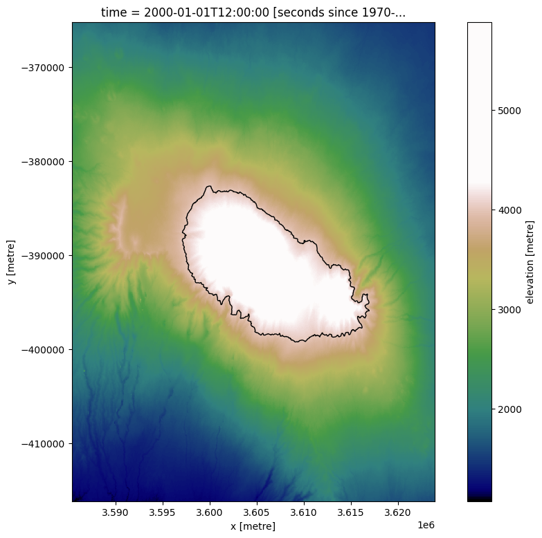
Extracting a single contour
Here, we extract a single 4000 m elevation contour:
[7]:
# Extract contours
contours_gdf = subpixel_contours(da=elevation_array,
                                 z_values=[4000])

# Print output
contours_gdf
Operating in multiple z-value, single array mode
[7]:
| z_value | geometry | |
|---|---|---|
| 0 | 4000 | MULTILINESTRING ((3609135 -399258.75, 3609105 ... |
This returns a geopandas.GeoDataFrame containing a single contour line feature with the z-value (i.e. elevation) given in a shapefile field named z_value. We can plot the extracted contour over the DEM:
[8]:
elevation_array.plot(size=9, cmap=cmap_terrain)
contours_gdf.plot(ax=plt.gca(), linewidth=1.0, color='black')
[8]:
<Axes: title={'center': 'time = 2000-01-01T12:00:00 [seconds since 1970-...'}, xlabel='x [metre]', ylabel='y [metre]'>
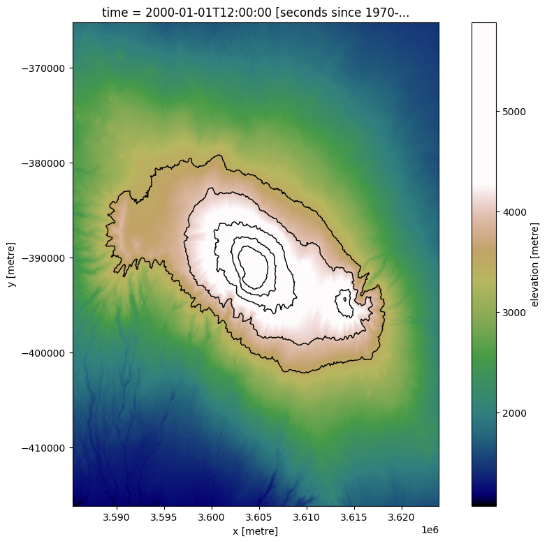
Extracting multiple contours
We can easily import multiple contours from a single array by supplying a list of z-values to extract. The function will then extract a contour for each value in z_values, skipping any contour elevation that is not found in the array.
[9]:
# List of elevations to extract
z_values = [3500, 4000, 4500, 5000, 5500]

# Extract contours
contours_gdf = subpixel_contours(da=elevation_array,
                                 z_values=z_values)

# Plot extracted contours over the DEM
elevation_array.plot(size=9, cmap=cmap_terrain)
contours_gdf.plot(ax=plt.gca(), linewidth=1.0, color='black')
Operating in multiple z-value, single array mode
[9]:
<Axes: title={'center': 'time = 2000-01-01T12:00:00 [seconds since 1970-...'}, xlabel='x [metre]', ylabel='y [metre]'>
Custom shapefile attributes
By default, the shapefile includes a single z_value attribute field with one feature per input value in z_values. We can instead pass custom attributes to the output shapefile using the attribute_df parameter. For example, we might want a custom column called elev_km with heights in Kilometres (km) instead of metres (m), and a location column giving the location, Mt Kilamanjaro (KLJ).
We can achieve this by first creating a pandas.DataFrame with column names giving the name of the attribute we want included with our contour features, and one row of values for each number in z_values:
[10]:
# Elevation values to extract in metres
z_values = [2000, 3000, 5500]

# Set up attribute dataframe (one row per elevation value above)
attribute_df = pd.DataFrame({'elev_km': [2, 3, 5.5],
                             'location': ['KLJ1', 'KLJ2', 'KLJ3']})

# Print output
attribute_df.head()
[10]:
| elev_km | location | |
|---|---|---|
| 0 | 2.0 | KLJ1 |
| 1 | 3.0 | KLJ2 |
| 2 | 5.5 | KLJ3 |
We can now extract contours, and the resulting contour features will include the attributes we created above:
[11]:
# Extract contours with custom attribute fields:
contours_gdf = subpixel_contours(da=elevation_array,
                                 z_values=z_values,
                                 attribute_df=attribute_df)

# Print output
contours_gdf.head()
Operating in multiple z-value, single array mode
[11]:
| z_value | elev_km | location | geometry | |
|---|---|---|---|---|
| 0 | 2000 | 2.0 | KLJ1 | MULTILINESTRING ((3585345 -367545, 3585375 -36... |
| 1 | 3000 | 3.0 | KLJ2 | MULTILINESTRING ((3609975 -405387, 3609945 -40... |
| 2 | 5500 | 5.5 | KLJ3 | MULTILINESTRING ((3604575 -393350, 3604545 -39... |
Exporting contours to file
To export the resulting contours to file, use the output_path parameter. The function supports two output file formats:
GeoJSON (.geojson)
Shapefile (.shp)
[12]:
subpixel_contours(da=elevation_array,
                  z_values=z_values,
                  output_path='output_contours.geojson')
Operating in multiple z-value, single array mode
Writing contours to output_contours.geojson
[12]:
| z_value | geometry | |
|---|---|---|
| 0 | 2000 | MULTILINESTRING ((3585345 -367545, 3585375 -36... |
| 1 | 3000 | MULTILINESTRING ((3609975 -405387, 3609945 -40... |
| 2 | 5500 | MULTILINESTRING ((3604575 -393350, 3604545 -39... |
Contours from non-elevation datasets in ‘single z-value, multiple arrays’ mode
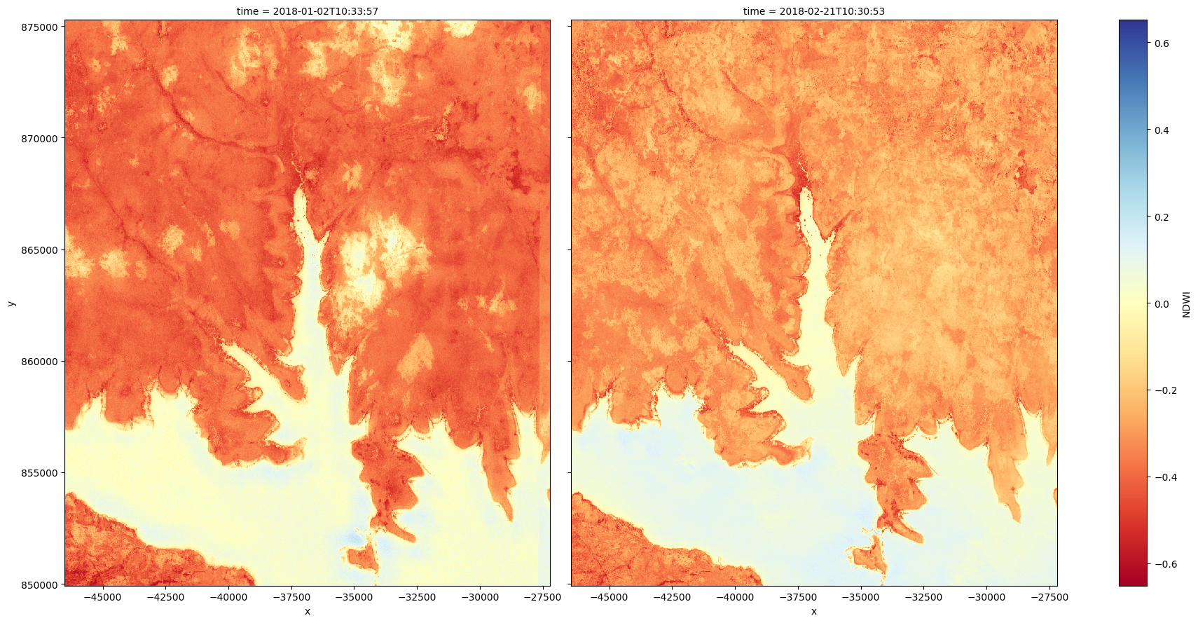
As well as extracting multiple contours from a single two-dimensional array, subpixel_contours also allows you to extract a single z-value from every array along a specified dimension in a multi-dimensional array. This can be useful for comparing the changes in the landscape across time. The input multi-dimensional array does not need to be elevation data: contours can be extracted from any type of data.
For example, we can use the function to extract the boundary between land and water (for a more in-depth analysis using contour extraction to monitor coastal erosion, see this notebook). First, we will load in a time series of Sentinel-2 imagery and calculate a simple Normalized Difference Water Index (NDWI) on two images. This index will have high values where a pixel is likely to be open water (e.g. NDWI > 0, coloured in blue below):
[13]:
# Set up a datacube query to load data for
# first provide a new location (Lake Volta in Ghana)
lat, lon = 6.777, -0.382
buffer = 0.1

#set-up a query
query = {
        'x': (lon-buffer, lon+buffer),
        'y': (lat+buffer, lat-buffer),
         'time': ('2018-01-01', '2018-02-25'),
         'measurements': ['nir_1', 'green'],
         'output_crs': 'EPSG:6933',
         'resolution': (-20, 20)}

# Load Sentinel 2 data
s2_ds = dc.load(product='s2_l2a',
                group_by='solar_day',
                progress_cbk=with_ui_cbk(),
                **query)
s2_ds
[13]:
<xarray.Dataset> Size: 54MB
Dimensions:      (time: 11, y: 1268, x: 966)
Coordinates:
  * time         (time) datetime64[ns] 88B 2018-01-02T10:33:57 ... 2018-02-21...
  * y            (y) float64 10kB 8.753e+05 8.752e+05 ... 8.5e+05 8.499e+05
  * x            (x) float64 8kB -4.651e+04 -4.649e+04 ... -2.723e+04 -2.721e+04
    spatial_ref  int32 4B 6933
Data variables:
    nir_1        (time, y, x) uint16 27MB 2120 2216 2202 2188 ... 720 716 753
    green        (time, y, x) uint16 27MB 1062 1090 1082 1068 ... 906 904 916
Attributes:
    crs:           EPSG:6933
grid_mapping: spatial_refCalculate NDWI on the first and last image in the dataset
[14]:
s2_ds = calculate_indices(s2_ds.isel(time=[0, -1]),
                          index='NDWI',
                          satellite_mission='s2'
                         )


# Plot the two images side by size
s2_ds.NDWI.plot(col='time', cmap='RdYlBu', size=9)
[14]:
<xarray.plot.facetgrid.FacetGrid at 0x7f2c6927b500>
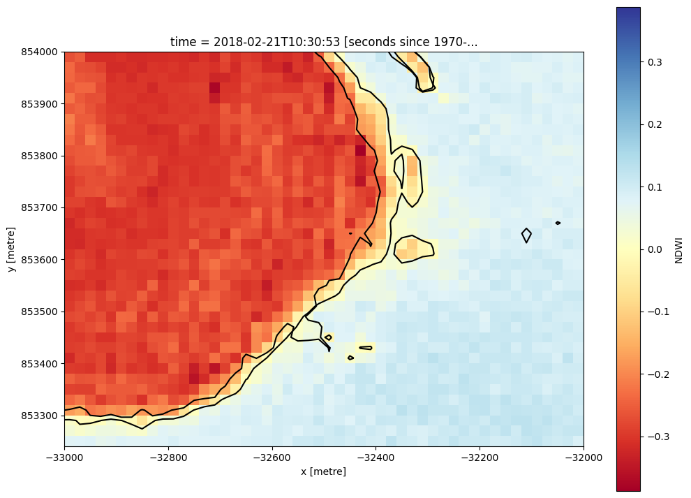
We can now identify the land-water boundary by extracting the 0 NDWI contour for each array in the dataset along the time dimension. By plotting the resulting contour lines for a zoomed in area, we can then start to compare phenomenon like lake levels across time.
[15]:
# Extract the 0 NDWI contour from both timesteps in the NDWI data
contours_gdf = subpixel_contours(da=s2_ds.NDWI,
                                 z_values=0,
                                 crs=s2_ds.geobox.crs,
                                 dim='time')

# Plot contours over the top of array
s2_ds.NDWI.isel(time=-1).sel(x = slice(-33000, -32000),
                        y = slice(854000, 853250)).plot(size = 9, cmap = 'RdYlBu')

contours_gdf.plot(ax = plt.gca(), linewidth = 1.5, color = 'black')
Operating in single z-value, multiple arrays mode
[15]:
<Axes: title={'center': 'time = 2018-02-21T10:30:53 [seconds since 1970-...'}, xlabel='x [metre]', ylabel='y [metre]'>
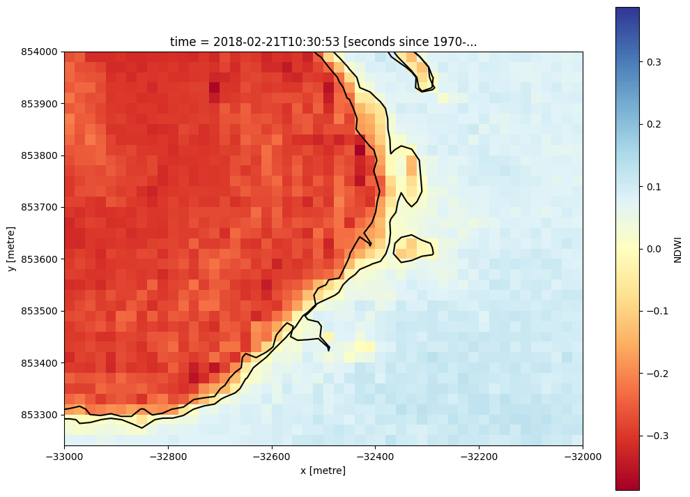
Dropping small contours
Contours produced by subpixel_contours can include many small features. We can optionally choose to extract only contours larger than a certain number of vertices using the min_vertices parameter. This can be useful for focusing on large contours, and remove possible noise in a dataset. Here we set min_vertices=10 to keep only contours with at least 10 vertices. Observe the small waterbody in the bottom-left of the image disappear:
[16]:
# Extract the 0 NDWI contour from both timesteps in the NDWI data
contours_gdf = subpixel_contours(da=s2_ds.NDWI,
                                 z_values=0,
                                 crs=s2_ds.geobox.crs,
                                 min_vertices=10)

# Plot contours over the top of array
# Plot contours over the top of array
s2_ds.NDWI.isel(time=-1).sel(x = slice(-33000, -32000),
                        y = slice(854000, 853250)).plot(size = 9, cmap = 'RdYlBu')

contours_gdf.plot(ax = plt.gca(), linewidth = 1.5, color = 'black')
Operating in single z-value, multiple arrays mode
[16]:
<Axes: title={'center': 'time = 2018-02-21T10:30:53 [seconds since 1970-...'}, xlabel='x [metre]', ylabel='y [metre]'>
Additional information
License: The code in this notebook is licensed under the Apache License, Version 2.0. Digital Earth Africa data is licensed under the Creative Commons by Attribution 4.0 license.
Contact: If you need assistance, please post a question on the Open Data Cube Slack channel or on the GIS Stack Exchange using the open-data-cube tag (you can view previously asked questions here). If you would like to report an issue with this notebook, you can file one on
Github.
Compatible datacube version:
[17]:
print(datacube.__version__)
1.8.20
Last Tested:
[18]:
from datetime import datetime
datetime.today().strftime('%Y-%m-%d')
[18]:
'2025-01-15'