Calculating band indices

• Products used: s2_l2a

Keywords data used; sentinel-2, band index; NDVI, band index; NDWI, band index; MNDWI

Background

Remote sensing indices are combinations of spectral bands used to highlight features in the data and the underlying landscape. For example, one of the most commonly used indices is the Normalised Difference Vegetation Index (NDVI), which uses the ratio of the red and near-infrared (NIR) band to highlight healthy vegetation (see here for a deeper explanation). Using Digital Earth Africa’s archive of analysis-ready satellite data, we can easily calculate a wide range of remote sensing indices that can be used to assist in mapping and monitoring features like vegetation and water consistently through time, or as inputs to machine learning or classification algorithms.

Description

This notebook demonstrates how to:

• Calculate an index manually using xarray

• Calculate one or multiple indices using the function calculate_indices from deafrica_bandindices.py

---

Getting started

To run this analysis, run all the cells in the notebook, starting with the “Load packages” cell.

Load packages

%matplotlib inline

import datacube
import matplotlib.pyplot as plt
import xarray as xr

from deafrica_tools.datahandling import load_ard, mostcommon_crs
from deafrica_tools.plotting import rgb
from deafrica_tools.bandindices import calculate_indices

Connect to the datacube

dc = datacube.Datacube(app='Calculating_band_indices')

Create a query and load satellite data

To demonstrate how to compute a remote sensing index, we first need to load in a time series of satellite data for an area. We will use data from the Sentinel-2 satellite:

lat, lon = 13.94, -16.54
buffer = 0.125

# Create a reusable query
query = {
    'x': (lon-buffer, lon+buffer),
    'y': (lat+buffer, lat-buffer),
    'time': ('2019-06', '2020-06'),
    'resolution': (-30, 30)
}

# Identify the most common projection system in the input query
output_crs = mostcommon_crs(dc=dc, product='s2_l2a', query=query)

# Load available data from Sentinel-2 and filter to retain only times
# with at least 99% good data
ds = load_ard(dc=dc,
              products=['s2_l2a'],
              min_gooddata=0.99,
              measurements=['red', 'green', 'blue', 'swir_1', 'swir_2', 'nir', 'nir_2'],
              output_crs=output_crs,
              **query)

Using pixel quality parameters for Sentinel 2
Finding datasets
    s2_l2a
Counting good quality pixels for each time step

CPLReleaseMutex: Error = 1 (Operation not permitted)

Filtering to 4 out of 78 time steps with at least 99.0% good quality pixels
Applying pixel quality/cloud mask
Loading 4 time steps

It is highly recommended to load data with load_ard when calculating indices, and when using the calculate_indices function introduced below. This is because load_ard performs the necessary data cleaning and scaling for more robust index results.

print(ds)

<xarray.Dataset>
Dimensions:      (time: 4, y: 928, x: 907)
Coordinates:
  * time         (time) datetime64[ns] 2019-10-20T11:47:38 ... 2020-03-18T11:...
  * y            (y) float64 1.556e+06 1.556e+06 ... 1.528e+06 1.528e+06
  * x            (x) float64 3.2e+05 3.201e+05 3.201e+05 ... 3.472e+05 3.472e+05
    spatial_ref  int32 32628
Data variables:
    red          (time, y, x) float32 2.067e+03 1e+03 ... 1.899e+03 1.93e+03
    green        (time, y, x) float32 1.707e+03 1.065e+03 ... 1.337e+03
    blue         (time, y, x) float32 896.0 452.0 520.0 ... 1.009e+03 993.0
    swir_1       (time, y, x) float32 4.049e+03 3.072e+03 ... 4.834e+03
    swir_2       (time, y, x) float32 3.372e+03 2.174e+03 ... 4.112e+03
    nir          (time, y, x) float32 4.196e+03 4.068e+03 ... 2.842e+03
    nir_2        (time, y, x) float32 4.361e+03 4.318e+03 ... 3.163e+03 3.05e+03
Attributes:
    crs:           epsg:32628
    grid_mapping:  spatial_ref

Plot the first image to see what our area looks like

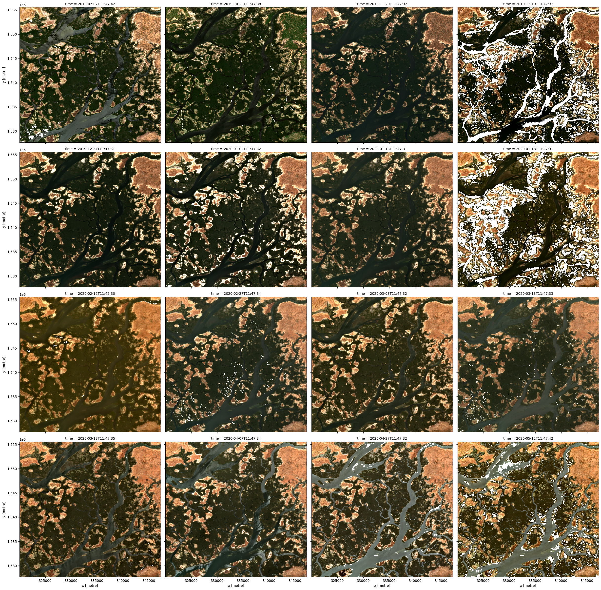
We can use the rgb function to plot the timesteps in our dataset as true colour RGB images:

# Plot as an RGB image

rgb(ds, col='time')

Manually calculate an index

One of the most commonly used remote sensing indices is the Normalised Difference Vegetation Index or NDVI. This index uses the ratio of the red and near-infrared (NIR) bands to identify live green vegetation. The formula for NDVI is:

\[\begin{split}\begin{aligned} \text{NDVI} & = \frac{(\text{NIR} - \text{Red})}{(\text{NIR} + \text{Red})} \\ \end{aligned}\end{split}\]

When interpreting this index, high values indicate vegetation, and low values indicate soil or water.

# Calculate NDVI using the formula above
ds['NDVI_manual'] = (ds.nir - ds.red) / (ds.nir + ds.red)

# Plot the results for one time step to see what they look like:
ds.NDVI_manual.plot(col='time', vmin=-0.50, vmax=0.8, cmap='RdYlGn')

<xarray.plot.facetgrid.FacetGrid at 0x7f7a603b9d60>

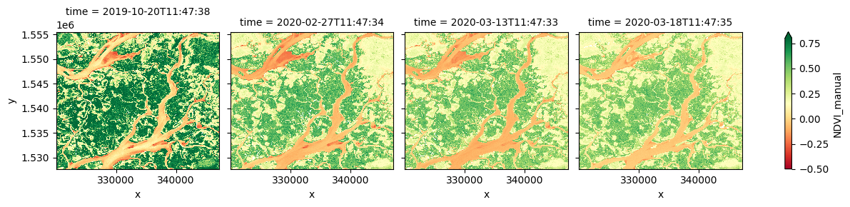
In the image above, vegetation shows up as green (NDVI > 0). Sand shows up as yellow (NDVI ~ 0) and water shows up as red (NDVI < 0).

Use the calculate_indices function to calculate an index

The calculate_indices function provides an easier way to calculate a wide range of remote sensing indices, including:

• ASI (Artificial Surface Index, Yongquan Zhao & Zhe Zhu 2022)

• AWEI_ns (Automated Water Extraction Index,no shadows, Feyisa 2014)

• AWEI_sh (Automated Water Extraction Index,shadows, Feyisa 2014)

• BAEI (Built-Up Area Extraction Index, Bouzekri et al. 2015)

• BAI (Burn Area Index, Martin 1998)

• BSI (Bare Soil Index, Rikimaru et al. 2002)

• BUI (Built-Up Index, He et al. 2010)

• CMR (Clay Minerals Ratio, Drury 1987)

• ENDISI (Enhanced Normalised Difference for Impervious Surfaces Index, Chen et al. 2019)

• EVI (Enhanced Vegetation Index, Huete 2002)

• FMR (Ferrous Minerals Ratio, Segal 1982)

• IOR (Iron Oxide Ratio, Segal 1982)

• LAI (Leaf Area Index, Boegh 2002)

• MBI (Modified Bare Soil Index, Nguyen et al. 2021)

• MNDWI (Modified Normalised Difference Water Index, Xu 1996)

• MSAVI (Modified Soil Adjusted Vegetation Index, Qi et al. 1994)

• NBI (New Built-Up Index, Jieli et al. 2010)

• NBR (Normalised Burn Ratio, Lopez Garcia 1991)

• NDBI (Normalised Difference Built-Up Index, Zha 2003)

• NDCI (Normalised Difference Chlorophyll Index, Mishra & Mishra, 2012)

• NDMI (Normalised Difference Moisture Index, Gao 1996)

• NDSI (Normalised Difference Snow Index, Hall 1995)

• NDTI (Normalised Difference Turbidity Index, Lacaux et al. 2007)

• NDVI (Normalised Difference Vegetation Index, Rouse 1973)

• NDWI (Normalised Difference Water Index, McFeeters 1996)

• SAVI (Soil Adjusted Vegetation Index, Huete 1988)

• TCB (Tasseled Cap Brightness, Crist 1985)

• TCG (Tasseled Cap Greeness, Crist 1985)

• TCW (Tasseled Cap Wetness, Crist 1985)

• WI (Water Index, Fisher 2016)

The calculate_indices function can be found in the deafrica_tools.bandindices script. This script provides all required band math involved in creating each index and is worth a look.

Using calculate_indices to get the same result

The function provides a simple way to calculate band indices without needing to explicitly write code for the band math.

calculate_indices(ds, index=['NDVI'], satellite_mission='s2')

<xarray.Dataset>
Dimensions:      (time: 4, y: 928, x: 907)
Coordinates:
  * time         (time) datetime64[ns] 2019-10-20T11:47:38 ... 2020-03-18T11:...
  * y            (y) float64 1.556e+06 1.556e+06 ... 1.528e+06 1.528e+06
  * x            (x) float64 3.2e+05 3.201e+05 3.201e+05 ... 3.472e+05 3.472e+05
    spatial_ref  int32 32628
Data variables:
    red          (time, y, x) float32 2.067e+03 1e+03 ... 1.899e+03 1.93e+03
    green        (time, y, x) float32 1.707e+03 1.065e+03 ... 1.337e+03
    blue         (time, y, x) float32 896.0 452.0 520.0 ... 1.009e+03 993.0
    swir_1       (time, y, x) float32 4.049e+03 3.072e+03 ... 4.834e+03
    swir_2       (time, y, x) float32 3.372e+03 2.174e+03 ... 4.112e+03
    nir          (time, y, x) float32 4.196e+03 4.068e+03 ... 2.842e+03
    nir_2        (time, y, x) float32 4.361e+03 4.318e+03 ... 3.163e+03 3.05e+03
    NDVI_manual  (time, y, x) float32 0.3399 0.6054 0.6021 ... 0.2269 0.1911
    NDVI         (time, y, x) float32 0.3399 0.6054 0.6021 ... 0.2269 0.1911
Attributes:
    crs:           epsg:32628
    grid_mapping:  spatial_ref

xarray.Dataset

• Dimensions:
  • time: 4
  • y: 928
  • x: 907
• Coordinates: (4)
  • time
    (time)
    datetime64[ns]
    2019-10-20T11:47:38 ... 2020-03-...

    units :

    seconds since 1970-01-01 00:00:00

    array(['2019-10-20T11:47:38.000000000', '2020-02-27T11:47:34.000000000',
           '2020-03-13T11:47:33.000000000', '2020-03-18T11:47:35.000000000'],
          dtype='datetime64[ns]')

  • y
    (y)
    float64
    1.556e+06 1.556e+06 ... 1.528e+06

    units :

    metre

    resolution :

    -30.0

    crs :

    epsg:32628

    array([1555545., 1555515., 1555485., ..., 1527795., 1527765., 1527735.])

  • x
    (x)
    float64
    3.2e+05 3.201e+05 ... 3.472e+05

    units :

    metre

    resolution :

    30.0

    crs :

    epsg:32628

    array([320025., 320055., 320085., ..., 347145., 347175., 347205.])

  • spatial_ref
    ()
    int32
    32628

    spatial_ref :

    PROJCS["WGS 84 / UTM zone 28N",GEOGCS["WGS 84",DATUM["WGS_1984",SPHEROID["WGS 84",6378137,298.257223563,AUTHORITY["EPSG","7030"]],AUTHORITY["EPSG","6326"]],PRIMEM["Greenwich",0,AUTHORITY["EPSG","8901"]],UNIT["degree",0.0174532925199433,AUTHORITY["EPSG","9122"]],AUTHORITY["EPSG","4326"]],PROJECTION["Transverse_Mercator"],PARAMETER["latitude_of_origin",0],PARAMETER["central_meridian",-15],PARAMETER["scale_factor",0.9996],PARAMETER["false_easting",500000],PARAMETER["false_northing",0],UNIT["metre",1,AUTHORITY["EPSG","9001"]],AXIS["Easting",EAST],AXIS["Northing",NORTH],AUTHORITY["EPSG","32628"]]

    grid_mapping_name :

    transverse_mercator

    array(32628, dtype=int32)

• Data variables: (9)
  • red
    (time, y, x)
    float32
    2.067e+03 1e+03 ... 1.93e+03

    units :

    1

    nodata :

    0

    crs :

    epsg:32628

    grid_mapping :

    spatial_ref

    array([[[2067., 1000., 1000., ..., 2011., 2623., 2642.],
            [1439., 1037.,  876., ..., 1105., 1853., 1983.],
            [ 605.,  813.,  945., ..., 1798., 2397., 1664.],
            ...,
            [ 327.,  323.,  310., ...,  658.,  932.,  825.],
            [ 315.,  328.,  320., ...,  738., 1121., 1009.],
            [ 336.,  316.,  363., ...,  758.,  836., 1052.]],
    
           [[2730., 2242., 2421., ..., 2360., 2932., 2714.],
            [2071., 2185., 2098., ..., 1991., 2271., 2514.],
            [2290., 2405., 2471., ..., 2237., 2606., 2383.],
            ...,
            [ 510.,  514.,  519., ..., 1846., 1940., 1768.],
            [ 520.,  515.,  511., ..., 1836., 1902., 1834.],
            [ 523.,  518.,  544., ..., 1803., 1795., 1835.]],
    
           [[2734., 2303., 2450., ..., 2579., 2733., 2644.],
            [2020., 2394., 2029., ..., 2065., 2355., 2489.],
            [2493., 2482., 2627., ..., 2283., 2623., 2388.],
            ...,
            [ 545.,  537.,  548., ..., 1932., 2008., 1882.],
            [ 545.,  550.,  524., ..., 1905., 1953., 1878.],
            [ 555.,  551.,  563., ..., 1901., 1852., 1899.]],
    
           [[2688., 2292., 2410., ..., 2525., 2715., 2561.],
            [2089., 2301., 2035., ..., 2096., 2341., 2443.],
            [2391., 2437., 2506., ..., 2280., 2555., 2365.],
            ...,
            [ 583.,  584.,  587., ..., 1956., 2031., 1854.],
            [ 594.,  585.,  577., ..., 1917., 1980., 1900.],
            [ 592.,  586.,  612., ..., 1917., 1899., 1930.]]], dtype=float32)

  • green
    (time, y, x)
    float32
    1.707e+03 1.065e+03 ... 1.337e+03

    units :

    1

    nodata :

    0

    crs :

    epsg:32628

    grid_mapping :

    spatial_ref

    array([[[1707., 1065., 1143., ..., 1665., 2170., 2190.],
            [1287., 1147., 1016., ..., 1045., 1540., 1663.],
            [ 856., 1005., 1158., ..., 1486., 2011., 1419.],
            ...,
            [ 463.,  473.,  457., ...,  727.,  899.,  817.],
            [ 463.,  455.,  449., ...,  710.,  979.,  888.],
            [ 499.,  493.,  488., ...,  761.,  772.,  904.]],
    
           [[1931., 1545., 1686., ..., 1755., 2097., 1974.],
            [1470., 1514., 1454., ..., 1387., 1585., 1796.],
            [1558., 1636., 1735., ..., 1566., 1847., 1672.],
            ...,
            [ 572.,  580.,  604., ..., 1248., 1357., 1220.],
            [ 591.,  588.,  575., ..., 1262., 1361., 1278.],
            [ 586.,  603.,  585., ..., 1247., 1269., 1272.]],
    
           [[1940., 1586., 1724., ..., 1892., 1979., 1866.],
            [1436., 1638., 1441., ..., 1438., 1649., 1743.],
            [1692., 1695., 1845., ..., 1576., 1835., 1652.],
            ...,
            [ 585.,  594.,  616., ..., 1344., 1449., 1331.],
            [ 596.,  601.,  578., ..., 1351., 1406., 1333.],
            [ 596.,  608.,  589., ..., 1326., 1316., 1324.]],
    
           [[1910., 1618., 1719., ..., 1862., 1911., 1844.],
            [1507., 1636., 1502., ..., 1481., 1643., 1731.],
            [1687., 1703., 1769., ..., 1593., 1797., 1658.],
            ...,
            [ 658.,  658.,  668., ..., 1391., 1451., 1332.],
            [ 652.,  670.,  638., ..., 1353., 1408., 1351.],
            [ 655.,  655.,  663., ..., 1344., 1332., 1337.]]], dtype=float32)

  • blue
    (time, y, x)
    float32
    896.0 452.0 ... 1.009e+03 993.0

    units :

    1

    nodata :

    0

    crs :

    epsg:32628

    grid_mapping :

    spatial_ref

    array([[[ 896.,  452.,  520., ..., 1065., 1474., 1588.],
            [ 619.,  506.,  451., ...,  576., 1046., 1173.],
            [ 333.,  406.,  501., ..., 1004., 1394.,  960.],
            ...,
            [ 187.,  195.,  193., ...,  348.,  504.,  434.],
            [ 197.,  205.,  199., ...,  372.,  625.,  529.],
            [ 214.,  195.,  239., ...,  427.,  450.,  549.]],
    
           [[1106.,  921., 1048., ..., 1171., 1453., 1388.],
            [ 863.,  969.,  915., ...,  971., 1106., 1237.],
            [ 978., 1041., 1104., ..., 1070., 1275., 1186.],
            ...,
            [ 389.,  383.,  383., ...,  903., 1003.,  854.],
            [ 386.,  385.,  382., ...,  915.,  994.,  928.],
            [ 387.,  376.,  401., ...,  913.,  928.,  925.]],
    
           [[1093.,  935., 1063., ..., 1270., 1322., 1274.],
            [ 866., 1004.,  877., ...,  961., 1118., 1205.],
            [1051., 1053., 1157., ..., 1047., 1237., 1129.],
            ...,
            [ 388.,  370.,  385., ...,  967., 1059.,  930.],
            [ 387.,  386.,  372., ...,  988., 1029.,  950.],
            [ 405.,  388.,  384., ...,  971.,  945.,  937.]],
    
           [[1174., 1020., 1112., ..., 1282., 1369., 1314.],
            [ 975., 1073.,  981., ..., 1041., 1166., 1230.],
            [1103., 1109., 1183., ..., 1112., 1264., 1180.],
            ...,
            [ 472.,  467.,  476., ..., 1031., 1117.,  962.],
            [ 463.,  473.,  470., ..., 1034., 1081., 1002.],
            [ 485.,  475.,  494., ..., 1030., 1009.,  993.]]], dtype=float32)

  • swir_1
    (time, y, x)
    float32
    4.049e+03 3.072e+03 ... 4.834e+03

    units :

    1

    nodata :

    0

    crs :

    epsg:32628

    grid_mapping :

    spatial_ref

    array([[[4049., 3072., 3083., ..., 4242., 4690., 4356.],
            [3498., 3216., 2818., ..., 3411., 4006., 3906.],
            [2528., 2803., 2931., ..., 3779., 4280., 3733.],
            ...,
            [ 890.,  902.,  879., ..., 2909., 3291., 3189.],
            [ 899.,  919.,  874., ..., 2950., 3485., 3359.],
            [ 878.,  890.,  900., ..., 2989., 3119., 3443.]],
    
           [[5096., 4774., 4858., ..., 4972., 5355., 5170.],
            [4471., 4690., 4531., ..., 4529., 4837., 5074.],
            [4649., 4764., 4782., ..., 4724., 5147., 5030.],
            ...,
            [ 936.,  960.,  949., ..., 4666., 4769., 4536.],
            [ 966.,  984.,  965., ..., 4692., 4780., 4639.],
            [ 955.,  964.,  993., ..., 4595., 4633., 4671.]],
    
           [[5073., 4857., 4837., ..., 5016., 5266., 5102.],
            [4565., 4810., 4636., ..., 4590., 4963., 5104.],
            [4937., 4801., 4969., ..., 4801., 5179., 5011.],
            ...,
            [ 892.,  899.,  910., ..., 4801., 4891., 4657.],
            [ 925.,  933.,  907., ..., 4795., 4866., 4815.],
            [ 881.,  915.,  898., ..., 4699., 4705., 4767.]],
    
           [[4971., 4785., 4826., ..., 5104., 5321., 5107.],
            [4487., 4799., 4503., ..., 4682., 4946., 5097.],
            [4778., 4829., 4890., ..., 4808., 5165., 5021.],
            ...,
            [1129., 1123., 1094., ..., 4948., 5005., 4733.],
            [1118., 1128., 1106., ..., 4908., 5018., 4881.],
            [1153., 1114., 1148., ..., 4780., 4802., 4834.]]], dtype=float32)

  • swir_2
    (time, y, x)
    float32
    3.372e+03 2.174e+03 ... 4.112e+03

    units :

    1

    nodata :

    0

    crs :

    epsg:32628

    grid_mapping :

    spatial_ref

    array([[[3372., 2174., 2119., ..., 3716., 4042., 3637.],
            [2673., 2204., 1800., ..., 2683., 3073., 3075.],
            [1562., 1757., 1891., ..., 2929., 3485., 2779.],
            ...,
            [ 475.,  482.,  450., ..., 1955., 2464., 2281.],
            [ 485.,  490.,  464., ..., 2038., 2687., 2557.],
            [ 475.,  457.,  483., ..., 2066., 2260., 2615.]],
    
           [[4777., 4149., 4245., ..., 4316., 4799., 4516.],
            [3939., 4016., 3861., ..., 3600., 3992., 4198.],
            [3743., 3973., 4153., ..., 3854., 4413., 4092.],
            ...,
            [ 635.,  645.,  628., ..., 3734., 3999., 3730.],
            [ 637.,  652.,  634., ..., 3834., 4059., 3923.],
            [ 639.,  627.,  673., ..., 3757., 3816., 3929.]],
    
           [[4520., 4325., 4254., ..., 4130., 4394., 4170.],
            [3794., 4073., 3780., ..., 3498., 4007., 4099.],
            [3899., 4031., 4250., ..., 3804., 4247., 3895.],
            ...,
            [ 606.,  619.,  613., ..., 3834., 4007., 3814.],
            [ 616.,  628.,  604., ..., 3929., 4077., 3982.],
            [ 614.,  612.,  631., ..., 3759., 3791., 3896.]],
    
           [[4599., 4307., 4329., ..., 4299., 4661., 4308.],
            [3861., 4166., 3909., ..., 3708., 4131., 4207.],
            [4045., 4145., 4332., ..., 4000., 4387., 4064.],
            ...,
            [ 728.,  737.,  710., ..., 4180., 4370., 3985.],
            [ 722.,  743.,  716., ..., 4189., 4381., 4276.],
            [ 752.,  714.,  747., ..., 3978., 4011., 4112.]]], dtype=float32)

  • nir
    (time, y, x)
    float32
    4.196e+03 4.068e+03 ... 2.842e+03

    units :

    1

    nodata :

    0

    crs :

    epsg:32628

    grid_mapping :

    spatial_ref

    array([[[4196., 4068., 4026., ..., 4188., 4168., 4127.],
            [3825., 4018., 3914., ..., 3495., 3758., 3581.],
            [4325., 4108., 4262., ..., 3532., 3917., 3325.],
            ...,
            [1984., 2005., 2119., ..., 3076., 3008., 2973.],
            [1992., 2003., 2048., ..., 2785., 2889., 2707.],
            [1940., 2204., 1958., ..., 2752., 2768., 2739.]],
    
           [[3899., 3459., 3562., ..., 3855., 3959., 3935.],
            [3370., 3537., 3395., ..., 3165., 3487., 3640.],
            [3616., 3663., 3697., ..., 3290., 3668., 3631.],
            ...,
            [1612., 1637., 1740., ..., 2897., 2945., 2784.],
            [1647., 1667., 1626., ..., 2855., 2927., 2797.],
            [1548., 1698., 1562., ..., 2807., 2887., 2780.]],
    
           [[3937., 3550., 3626., ..., 3925., 3853., 3821.],
            [3356., 3657., 3407., ..., 3232., 3551., 3660.],
            [3780., 3652., 3788., ..., 3358., 3692., 3677.],
            ...,
            [1535., 1549., 1601., ..., 3021., 3057., 2895.],
            [1568., 1590., 1506., ..., 2925., 2946., 2824.],
            [1470., 1594., 1427., ..., 2881., 2964., 2840.]],
    
           [[3702., 3413., 3440., ..., 3781., 3715., 3681.],
            [3251., 3459., 3298., ..., 3225., 3470., 3572.],
            [3570., 3532., 3579., ..., 3282., 3563., 3589.],
            ...,
            [1602., 1604., 1648., ..., 3014., 3026., 2878.],
            [1617., 1628., 1570., ..., 2928., 3000., 2858.],
            [1573., 1659., 1523., ..., 2912., 3014., 2842.]]], dtype=float32)

  • nir_2
    (time, y, x)
    float32
    4.361e+03 4.318e+03 ... 3.05e+03

    units :

    1

    nodata :

    0

    crs :

    epsg:32628

    grid_mapping :

    spatial_ref

    array([[[4361., 4318., 4312., ..., 4411., 4471., 4268.],
            [4139., 4179., 4276., ..., 3755., 4072., 3832.],
            [4562., 4248., 4509., ..., 3795., 4145., 3658.],
            ...,
            [2119., 2120., 2283., ..., 3392., 3313., 3216.],
            [2245., 2233., 2223., ..., 3119., 3128., 3061.],
            [2165., 2383., 2126., ..., 3002., 3045., 3023.]],
    
           [[3899., 3565., 3659., ..., 3853., 4050., 3995.],
            [3535., 3639., 3574., ..., 3312., 3598., 3709.],
            [3747., 3623., 3723., ..., 3412., 3740., 3738.],
            ...,
            [1659., 1698., 1795., ..., 3077., 3093., 2918.],
            [1716., 1748., 1649., ..., 3023., 3035., 2921.],
            [1602., 1752., 1635., ..., 2960., 2998., 2937.]],
    
           [[3864., 3698., 3731., ..., 3883., 3988., 3920.],
            [3579., 3748., 3526., ..., 3339., 3632., 3736.],
            [3844., 3751., 3760., ..., 3461., 3732., 3773.],
            ...,
            [1514., 1547., 1641., ..., 3170., 3159., 2982.],
            [1619., 1612., 1531., ..., 3089., 3114., 2961.],
            [1511., 1640., 1485., ..., 3039., 3112., 2993.]],
    
           [[3604., 3609., 3618., ..., 3920., 3897., 3839.],
            [3430., 3663., 3480., ..., 3400., 3620., 3736.],
            [3625., 3654., 3664., ..., 3459., 3698., 3772.],
            ...,
            [1656., 1678., 1762., ..., 3200., 3203., 3021.],
            [1687., 1715., 1659., ..., 3129., 3152., 3082.],
            [1624., 1722., 1624., ..., 3110., 3163., 3050.]]], dtype=float32)

  • NDVI_manual
    (time, y, x)
    float32
    0.3399 0.6054 ... 0.2269 0.1911

    array([[[0.33993295, 0.605367  , 0.60206926, ..., 0.35118568,
             0.227507  , 0.21938248],
            [0.45326748, 0.58971316, 0.634238  , ..., 0.5195652 ,
             0.33951166, 0.28720346],
            [0.75456387, 0.6695793 , 0.6370271 , ..., 0.32532832,
             0.24073488, 0.33293244],
            ...,
            [0.7170056 , 0.7225086 , 0.7447509 , ..., 0.6475629 ,
             0.52690357, 0.5655608 ],
            [0.7269181 , 0.7185757 , 0.7297297 , ..., 0.5810389 ,
             0.44089776, 0.45694295],
            [0.7047452 , 0.74920636, 0.68720376, ..., 0.56809115,
             0.536071  , 0.4450013 ]],
    
           [[0.17634636, 0.21347132, 0.190707  , ..., 0.24054706,
             0.14903498, 0.18363664],
            [0.23874287, 0.23628102, 0.23611869, ..., 0.22769588,
             0.21118444, 0.18297042],
            [0.22451743, 0.20731707, 0.19876784, ..., 0.19051927,
             0.16927001, 0.20751579],
    ...
            [0.47596154, 0.485139  , 0.48999536, ..., 0.21986675,
             0.2071076 , 0.21205778],
            [0.48414576, 0.48598132, 0.48374385, ..., 0.21118012,
             0.20269443, 0.20119098],
            [0.45185184, 0.4862471 , 0.43417084, ..., 0.20493518,
             0.23089701, 0.1985651 ]],
    
           [[0.15868545, 0.1964943 , 0.17606838, ..., 0.19917539,
             0.15552099, 0.17942967],
            [0.217603  , 0.20104167, 0.2368273 , ..., 0.21217816,
             0.1942867 , 0.18769743],
            [0.1977856 , 0.18344781, 0.17633525, ..., 0.18015103,
             0.16475973, 0.20557608],
            ...,
            [0.46636155, 0.46617916, 0.47472036, ..., 0.21287726,
             0.19675697, 0.21639898],
            [0.46268657, 0.4713059 , 0.46250582, ..., 0.20866872,
             0.20481928, 0.2013451 ],
            [0.4531178 , 0.477951  , 0.42669788, ..., 0.2060468 ,
             0.22694892, 0.19111484]]], dtype=float32)

  • NDVI
    (time, y, x)
    float32
    0.3399 0.6054 ... 0.2269 0.1911

    array([[[0.33993298, 0.605367  , 0.6020692 , ..., 0.35118568,
             0.22750695, 0.21938246],
            [0.45326748, 0.5897131 , 0.634238  , ..., 0.51956517,
             0.3395117 , 0.28720343],
            [0.7545639 , 0.6695794 , 0.6370271 , ..., 0.32532832,
             0.24073488, 0.33293247],
            ...,
            [0.7170056 , 0.7225086 , 0.7447509 , ..., 0.64756286,
             0.52690357, 0.5655608 ],
            [0.7269181 , 0.71857566, 0.7297297 , ..., 0.5810389 ,
             0.44089773, 0.45694298],
            [0.7047452 , 0.74920636, 0.68720376, ..., 0.56809115,
             0.536071  , 0.44500136]],
    
           [[0.17634636, 0.21347132, 0.19070703, ..., 0.24054708,
             0.149035  , 0.18363664],
            [0.23874287, 0.23628104, 0.2361187 , ..., 0.22769588,
             0.21118441, 0.18297043],
            [0.22451745, 0.20731705, 0.19876786, ..., 0.19051926,
             0.16927001, 0.20751579],
    ...
            [0.47596157, 0.485139  , 0.48999533, ..., 0.21986674,
             0.2071076 , 0.21205778],
            [0.4841458 , 0.48598132, 0.48374382, ..., 0.21118009,
             0.20269446, 0.201191  ],
            [0.45185184, 0.48624706, 0.43417087, ..., 0.20493518,
             0.23089701, 0.19856511]],
    
           [[0.15868548, 0.19649431, 0.1760684 , ..., 0.19917542,
             0.15552099, 0.17942965],
            [0.21760298, 0.20104167, 0.2368273 , ..., 0.21217816,
             0.1942867 , 0.18769744],
            [0.19778562, 0.18344781, 0.17633522, ..., 0.18015105,
             0.16475976, 0.20557612],
            ...,
            [0.46636152, 0.46617913, 0.4747204 , ..., 0.21287726,
             0.19675697, 0.21639901],
            [0.46268654, 0.4713059 , 0.46250582, ..., 0.20866875,
             0.20481929, 0.20134513],
            [0.45311776, 0.47795102, 0.4266979 , ..., 0.20604682,
             0.22694893, 0.19111484]]], dtype=float32)

• Attributes: (2)

  crs :

  epsg:32628

  grid_mapping :

  spatial_ref

# Calculate NDVI using `calculate indices`
ds_ndvi = calculate_indices(ds, index='NDVI', satellite_mission='s2')

# Plot the results
ds_ndvi.NDVI.plot(col='time', vmin=-0.50, vmax=0.8, cmap='RdYlGn')

<xarray.plot.facetgrid.FacetGrid at 0x7f7a5c23c250>

Note: when using the calculate_indices function, it is important to set the satellite_mission parameter correctly. This is because different satellite missions use different names for the same bands, which can lead to invalid results if not accounted for. For Sentinel-2 , specify satellite_mission='s2'. For Landsat Collection 2, specify satellite_mission='ls'.

Using calculate_indices to calculate multiple indices at once

The calculate_indices function makes it straightforward to calculate multiple remote sensing indices in one line of code.

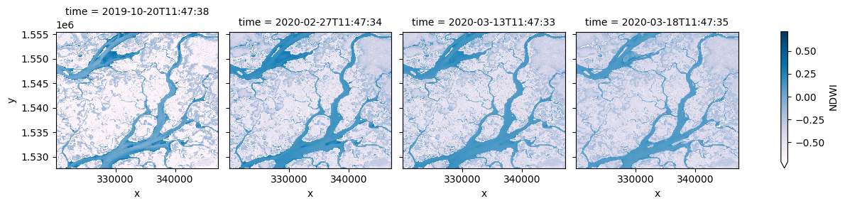
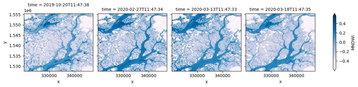
In the example below, we will calculate NDVI as well as two common water indices: the Normalised Difference Water Index (NDWI), and the Modified Normalised Difference Index (MNDWI). The new indices will appear in the list of data_variables below:

# Calculate multiple indices
ds_multi = calculate_indices(ds, index=['NDVI', 'NDWI', 'MNDWI'], satellite_mission='s2')

print(ds_multi)

<xarray.Dataset>
Dimensions:      (time: 4, y: 928, x: 907)
Coordinates:
  * time         (time) datetime64[ns] 2019-10-20T11:47:38 ... 2020-03-18T11:...
  * y            (y) float64 1.556e+06 1.556e+06 ... 1.528e+06 1.528e+06
  * x            (x) float64 3.2e+05 3.201e+05 3.201e+05 ... 3.472e+05 3.472e+05
    spatial_ref  int32 32628
Data variables:
    red          (time, y, x) float32 2.067e+03 1e+03 ... 1.899e+03 1.93e+03
    green        (time, y, x) float32 1.707e+03 1.065e+03 ... 1.337e+03
    blue         (time, y, x) float32 896.0 452.0 520.0 ... 1.009e+03 993.0
    swir_1       (time, y, x) float32 4.049e+03 3.072e+03 ... 4.834e+03
    swir_2       (time, y, x) float32 3.372e+03 2.174e+03 ... 4.112e+03
    nir          (time, y, x) float32 4.196e+03 4.068e+03 ... 2.842e+03
    nir_2        (time, y, x) float32 4.361e+03 4.318e+03 ... 3.163e+03 3.05e+03
    NDVI_manual  (time, y, x) float32 0.3399 0.6054 0.6021 ... 0.2269 0.1911
    NDVI         (time, y, x) float32 0.3399 0.6054 0.6021 ... 0.2269 0.1911
    NDWI         (time, y, x) float32 -0.4217 -0.585 -0.5577 ... -0.387 -0.3601
    MNDWI        (time, y, x) float32 -0.4069 -0.4851 ... -0.5657 -0.5667
Attributes:
    crs:           epsg:32628
    grid_mapping:  spatial_ref

# Plot the NDWI results
ds_multi.NDWI.plot(col='time', robust=True, cmap='PuBu')

<xarray.plot.facetgrid.FacetGrid at 0x7f7a5c21bb20>

# Plot the MNDWI results
ds_multi.MNDWI.plot(col='time', robust=True, cmap='PuBu')

<xarray.plot.facetgrid.FacetGrid at 0x7f7a44813340>

We can also drop the original satellite bands from the dataset using drop=True. The dataset produced below should now only include the new 'NDVI', 'NDWI', 'MNDWI' bands under data_variables:

# Calculate multiple indices and drop original bands
ds_drop = calculate_indices(ds, index=['NDVI', 'NDWI', 'MNDWI'], drop=True, satellite_mission='s2')
print(ds_drop)

Dropping bands ['red', 'green', 'blue', 'swir_1', 'swir_2', 'nir', 'nir_2', 'NDVI_manual']
<xarray.Dataset>
Dimensions:      (time: 4, y: 928, x: 907)
Coordinates:
  * time         (time) datetime64[ns] 2019-10-20T11:47:38 ... 2020-03-18T11:...
  * y            (y) float64 1.556e+06 1.556e+06 ... 1.528e+06 1.528e+06
  * x            (x) float64 3.2e+05 3.201e+05 3.201e+05 ... 3.472e+05 3.472e+05
    spatial_ref  int32 32628
Data variables:
    NDVI         (time, y, x) float32 0.3399 0.6054 0.6021 ... 0.2269 0.1911
    NDWI         (time, y, x) float32 -0.4217 -0.585 -0.5577 ... -0.387 -0.3601
    MNDWI        (time, y, x) float32 -0.4069 -0.4851 ... -0.5657 -0.5667
Attributes:
    crs:           epsg:32628
    grid_mapping:  spatial_ref

---

Additional information

License: The code in this notebook is licensed under the Apache License, Version 2.0. Digital Earth Africa data is licensed under the Creative Commons by Attribution 4.0 license.

Contact: If you need assistance, please post a question on the Open Data Cube Slack channel or on the GIS Stack Exchange using the open-data-cube tag (you can view previously asked questions here). If you would like to report an issue with this notebook, you can file one on Github.

Compatible datacube version:

print(datacube.__version__)

1.8.6

Last Tested:

from datetime import date
print(date.today())

2022-07-15