Image segmentation

• Products used: s2_l2a

Keywords data used; sentinel-2, analysis; machine learning, machine learning; image segmentation, data methods; composites, analysis; GEOBIA, band index; NDVI, data format; GeoTIFF

Background

In the last two decades, as the spatial resolution of satellite images has increased, remote sensing has begun to shift from a focus on pixel-based analysis towards Geographic Object-Based Image Analysis (GEOBIA), which aims to group pixels together into meaningful image-objects. There are two advantages to a GEOBIA worklow; one, we can reduce the ‘salt and pepper’ effect typical of classifying pixels; and two, we can increase the computational efficiency of our workflow by grouping pixels into fewer, larger, but meaningful objects. A review of the emerging trends in GEOBIA can be found in Chen et al. (2017).

Description

This notebook demonstrates a method for conducting image segmentation, which is a common image analysis technique used to transform a digital satellite image into objects. In brief, image segmentation aims to partition an image into segments, where each segment consists of a group of pixels with similar characteristics. Here we use the Quickshift algorithm, implemented through the python package scikit-image, to perform the image segmentation.

Getting started

To run this analysis, run all the cells in the notebook, starting with the “Load packages” cell.

Load packages

%matplotlib inline

import datacube
import xarray as xr
import numpy as np
import geopandas as gpd
import scipy
import matplotlib.pyplot as plt
from osgeo import gdal
from datacube.utils.cog import write_cog
from datacube.utils.geometry import Geometry
from skimage.segmentation import quickshift

from deafrica_tools.plotting import display_map
from deafrica_tools.areaofinterest import define_area
from deafrica_tools.bandindices import calculate_indices
from deafrica_tools.datahandling import load_ard, mostcommon_crs, array_to_geotiff

Connect to the datacube

dc = datacube.Datacube(app='Image_segmentation')

Analysis parameters

The following cell sets the parameters, which define the area of interest and the length of time to conduct the analysis over. The parameters are

• lat: The central latitude to analyse (e.g. 6.502).

• lon: The central longitude to analyse (e.g. -1.409).

• buffer: The number of square degrees to load around the central latitude and longitude. For reasonable loading times, set this as 0.1 or lower.

• time: The date range to analyse (e.g. ("2017-08-01", "2019-11-01")). For reasonable loading times, make sure the range spans less than 3 years. Note that Sentinel-2 data is only available after July 2015.

Select location

To define the area of interest, there are two methods available:

1. By specifying the latitude, longitude, and buffer. This method requires you to input the central latitude, central longitude, and the buffer value in square degrees around the center point you want to analyze. For example, lat = 10.338, lon = -1.055, and buffer = 0.1 will select an area with a radius of 0.1 square degrees around the point with coordinates (10.338, -1.055).

2. By uploading a polygon as a GeoJSON or Esri Shapefile. If you choose this option, you will need to upload the geojson or ESRI shapefile into the Sandbox using Upload Files button in the top left corner of the Jupyter Notebook interface. ESRI shapefiles must be uploaded with all the related files (.cpg, .dbf, .shp, .shx). Once uploaded, you can use the shapefile or geojson to define the area of interest. Remember to update the code to call the file you have uploaded.

To use one of these methods, you can uncomment the relevant line of code and comment out the other one. To comment out a line, add the "#" symbol before the code you want to comment out. By default, the first option which defines the location using latitude, longitude, and buffer is being used.

# Set the area of interest
# Method 1: Specify the latitude, longitude, and buffer
aoi = define_area(lat=-31.704, lon=18.523, buffer=0.03)

# Method 2: Use a polygon as a GeoJSON or Esri Shapefile.
# aoi = define_area(vector_path='aoi.shp')

#Create a geopolygon and geodataframe of the area of interest
geopolygon = Geometry(aoi["features"][0]["geometry"], crs="epsg:4326")
geopolygon_gdf = gpd.GeoDataFrame(geometry=[geopolygon], crs=geopolygon.crs)

# Get the latitude and longitude range of the geopolygon
lat_range = (geopolygon_gdf.total_bounds[1], geopolygon_gdf.total_bounds[3])
lon_range = (geopolygon_gdf.total_bounds[0], geopolygon_gdf.total_bounds[2])

# x = (lon - buffer, lon + buffer)
# y =  (lat + buffer, lat - buffer)

# Create a reusable query
query = {
    'x': lon_range,
    'y': lat_range,
    'time': ('2018-01', '2018-03'),
    'resolution': (-30, 30)
}

View the selected location

display_map(x=lon_range, y=lat_range)

Make this Notebook Trusted to load map: File -> Trust Notebook

Load Sentinel-2 data from the datacube

Here we are loading in a timeseries of Sentinel-2 satellite images through the datacube API using the load_ard function. This will provide us with some data to work with.

#find the most common UTM crs for the location
output_crs = mostcommon_crs(dc=dc, product='s2_l2a', query=query)

# Load available data
ds = load_ard(dc=dc,
              products=['s2_l2a'],
              measurements=['red', 'nir_1', 'swir_1', 'swir_2'],
              group_by='solar_day',
              output_crs=output_crs,
              **query)

# Print output data
print(ds)

Using pixel quality parameters for Sentinel 2
Finding datasets
    s2_l2a
Applying pixel quality/cloud mask
Loading 35 time steps

/usr/local/lib/python3.10/dist-packages/rasterio/warp.py:344: NotGeoreferencedWarning: Dataset has no geotransform, gcps, or rpcs. The identity matrix will be returned.
  _reproject(
/usr/local/lib/python3.10/dist-packages/rasterio/warp.py:344: NotGeoreferencedWarning: Dataset has no geotransform, gcps, or rpcs. The identity matrix will be returned.
  _reproject(

<xarray.Dataset>
Dimensions:      (time: 35, y: 227, x: 195)
Coordinates:
  * time         (time) datetime64[ns] 2018-01-01T08:42:22 ... 2018-03-30T08:...
  * y            (y) float64 6.493e+06 6.493e+06 ... 6.486e+06 6.486e+06
  * x            (x) float64 2.623e+05 2.624e+05 ... 2.681e+05 2.682e+05
    spatial_ref  int32 32734
Data variables:
    red          (time, y, x) float32 3.387e+03 2.899e+03 ... 1.366e+03
    nir_1        (time, y, x) float32 4.423e+03 3.662e+03 ... 2.583e+03
    swir_1       (time, y, x) float32 6.469e+03 5.326e+03 ... 3.069e+03
    swir_2       (time, y, x) float32 5.309e+03 4.276e+03 ... 2.153e+03
Attributes:
    crs:           epsg:32734
    grid_mapping:  spatial_ref

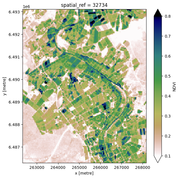
Combine observations into a noise-free statistical summary image

Individual remote sensing images can be affected by noisy and incomplete data (e.g. due to clouds). To produce cleaner images that we can feed into the image segmentation algorithm, we can create summary images, or composites, that combine multiple images into one image to reveal the ‘typical’ appearance of the landscape for a certain time period. In the code below, we take the noisy, incomplete satellite images we just loaded and calculate the mean Normalised Difference Vegetation Index (NDVI). The mean NDVI will be our input into the segmentation algorithm.

Calculate mean NDVI

# First we calculate NDVI on each image in the timeseries
ndvi = calculate_indices(ds, index='NDVI', satellite_mission='s2')

# For each pixel, calculate the mean NDVI throughout the whole timeseries
ndvi = ndvi.mean(dim='time', keep_attrs=True)

# Plot the results to inspect
ndvi.NDVI.plot(vmin=0.1, vmax=0.8, cmap='gist_earth_r', figsize=(7, 7))

<matplotlib.collections.QuadMesh at 0x7f3bc6880400>

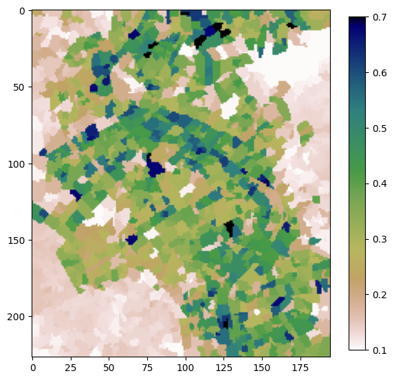
Quickshift Segmentation

Using the function quickshift from the python package scikit-image, we will conduct an image segmentation on the mean NDVI array. We then calculate a zonal mean across each segment using the input dataset. Our last step is to export our results as a GeoTIFF.

Follow the quickshift hyperlink above to see the input parameters to the algorithm, and the following link for an explanation of quickshift and other segmentation algorithms in scikit-image.

# Convert our mean NDVI xarray into a numpy array, we need
# to be explicit about the datatype to satisfy quickshift
input_array = ndvi.NDVI.values.astype(np.float64)

# Calculate the segments
segments = quickshift(input_array,
                      kernel_size=1,
                      convert2lab=False,
                      max_dist=2,
                      ratio=1.0)

# Calculate the zonal mean NDVI across the segments
segments_zonal_mean_qs = scipy.ndimage.mean(input=input_array,
                                            labels=segments,
                                            index=segments)

# Plot to see result
plt.figure(figsize=(7,7))
plt.imshow(segments_zonal_mean_qs, cmap='gist_earth_r', vmin=0.1, vmax=0.7)
plt.colorbar(shrink=0.9)

<matplotlib.colorbar.Colorbar at 0x7f3bc68bf610>

Export result to GeoTIFF

See this notebook for more info on writing GeoTIFFs to file.

transform = ds.geobox.transform.to_gdal()
projection = ds.geobox.crs.wkt

# Export the array
array_to_geotiff('segmented_meanNDVI_QS.tif',
                  segments_zonal_mean_qs,
                  geo_transform=transform,
                  projection=projection,
                  nodata_val=np.nan)

---

Additional information

License: The code in this notebook is licensed under the Apache License, Version 2.0. Digital Earth Africa data is licensed under the Creative Commons by Attribution 4.0 license.

Contact: If you need assistance, please post a question on the Open Data Cube Slack channel or on the GIS Stack Exchange using the open-data-cube tag (you can view previously asked questions here). If you would like to report an issue with this notebook, you can file one on Github.

Compatible datacube version:

print(datacube.__version__)

1.8.15

Last Tested:

from datetime import datetime
datetime.today().strftime('%Y-%m-%d')

'2023-08-14'