Applying WOfS Bitmasking
Products used: wofs_ls
Keywords data used; WOfS, data methods; wofs_fuser, analysis; masking
Background
The Water Observations from Space (WOfS) product shows water observed by Landsat satellites over Africa.
Individual water classified images are called Water Observation Feature Layers (WOFLs), and are created in a 1-to-1 relationship with the input satellite data. Hence there is one WOFL for each satellite dataset processed for the occurrence of water.
Description
This notebook explains both the structure of the WOFLs, and how you can use this for powerful and flexible image masking.
The data in a WOFL is stored as a bit field. This is a binary number, where each digit of the number is independantly set or not based on the presence (1) or absence (0) of a particular attribute (water, cloud, cloud shadow etc). In this way, the single decimal value associated to each pixel can provide information on a variety of features of that pixel.
The notebook demonstrates how to:
Load WOFL data for a given location and time period
Inspect the WOLF bit flag information
Use the WOFL bit flags to create a binary mask
Getting started
To run this analysis, run all the cells in the notebook, starting with the “Load packages” cell.
After finishing the analysis, you can modify some values in the “Analysis parameters” cell and re-run the analysis to load WOFLs for a different location or time period.
Load packages
[1]:
%matplotlib inline

import datacube
import numpy as np
import geopandas as gpd
import matplotlib.pyplot as plt
from datacube.utils import masking
from odc.geo.geom import Geometry

from deafrica_tools.plotting import display_map, plot_wofs
from deafrica_tools.datahandling import wofs_fuser, mostcommon_crs
from deafrica_tools.areaofinterest import define_area
Connect to the datacube
[2]:
dc = datacube.Datacube(app="Applying_WOfS_bitmasking")
Analysis parameters
To load WOFL data, we can first create a re-usable query that will define the spatial extent and time period we are interested in, as well as other important parameters that are used to correctly load the data.
Select location
To define the area of interest, there are two methods available:
By specifying the latitude, longitude, and buffer. This method requires you to input the central latitude, central longitude, and the buffer value in square degrees around the center point you want to analyze. For example,
lat = 10.338,lon = -1.055, andbuffer = 0.1will select an area with a radius of 0.1 square degrees around the point with coordinates (10.338, -1.055).By uploading a polygon as a
GeoJSON or Esri Shapefile. If you choose this option, you will need to upload the geojson or ESRI shapefile into the Sandbox using Upload Files button in the top left corner of the Jupyter Notebook interface. ESRI shapefiles must be uploaded with all the related files
 (.cpg, .dbf, .shp, .shx). Once uploaded, you can use the shapefile or geojson to define the area of interest. Remember to update the code to call the file you have uploaded.
To use one of these methods, you can uncomment the relevant line of code and comment out the other one. To comment out a line, add the "#" symbol before the code you want to comment out. By default, the first option which defines the location using latitude, longitude, and buffer is being used.
If running the notebook for the first time, keep the default settings below. This will demonstrate how the analysis works and provide meaningful results.
[3]:
# Method 1: Specify the latitude, longitude, and buffer
aoi = define_area(lat=-11.6216, lon=29.6987, buffer=0.175)

# Method 2: Use a polygon as a GeoJSON or Esri Shapefile.
# aoi = define_area(vector_path='aoi.shp')

#Create a geopolygon and geodataframe of the area of interest
geopolygon = Geometry(aoi["features"][0]["geometry"], crs="epsg:4326")
geopolygon_gdf = gpd.GeoDataFrame(geometry=[geopolygon], crs=geopolygon.crs)

# Get the latitude and longitude range of the geopolygon
lat_range = (geopolygon_gdf.total_bounds[1], geopolygon_gdf.total_bounds[3])
lon_range = (geopolygon_gdf.total_bounds[0], geopolygon_gdf.total_bounds[2])

# Create a reusable query
query = {
    'x': lon_range,
    'y': lat_range,
    'time': ('2018-10'),
    'resolution': (-30, 30)
}
View the selected location
[4]:
display_map(x=lon_range,y=lat_range)
[4]:
Load WOFL data
As WOFLs are created scene-by-scene, and some scenes overlap, it’s important when loading data to group_by solar day, and ensure that the data between scenes is combined correctly by using the WOfS fuse_func. This will merge observations taken on the same day, and ensure that important data isn’t lost when overlapping datasets are combined.
[5]:
# Load the data from the datacube
output_crs = mostcommon_crs(dc=dc, product='wofs_ls', query=query)

wofls = dc.load(product="wofs_ls",
                output_crs=output_crs,
                group_by="solar_day",
                fuse_func=wofs_fuser,
                collection_category='T1', #only grab good georeferenced scenes
                **query)
/home/jovyan/dev/deafrica-sandbox-notebooks/Tools/deafrica_tools/datahandling.py:739: UserWarning: Multiple UTM zones ['epsg:32636', 'epsg:32635'] were returned for this query. Defaulting to the most common zone: epsg:32636
  warnings.warn(
Plot the loaded WOFLs using the plot_wofs function
[6]:
plot_wofs(wofls.water, col='time', col_wrap=7);
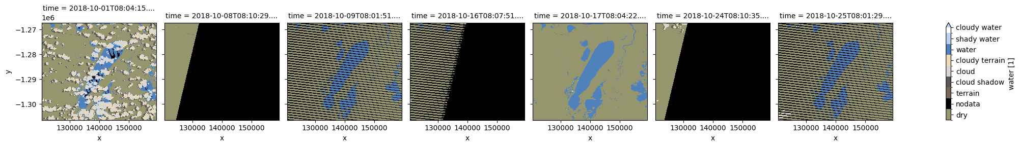
[7]:
# Select one image of interest (`time=4` selects the fifth observation)
wofl = wofls.isel(time=4)
Understanding the WOFLs
As mentioned above, WOFLs are stored as a binary number, where each digit of the number is independantly set or not based on the presence (1) or absence (0) of a particular feature. Below is a breakdown of which bits represent which features, along with the decimal value associated with that bit being set to true.
Attribute |
Bit / position |
Decimal value |
|---|---|---|
No data |
0: |
1 |
Non contiguous |
1: |
2 |
Sea (not used) |
2: |
4 |
Terrain or low solar angle |
3: |
8 |
High slope |
4: |
16 |
Cloud shadow |
5: |
32 |
Cloud |
6: |
64 |
Water |
7: |
128 |
The values in the above plots are the decimal representation of the combination of set flags. For example a value of 136 indicates water (128) AND terrain shadow / low solar angle (8) were observed for the pixel, whereas a value of 144 would indicate water (128) AND high slope (16).
This flag information is available inside the loaded data and can be visualised as below
[8]:
# Display details of available flags
flags = masking.describe_variable_flags(wofls)
flags["bits"] = flags["bits"].astype(str)
flags.sort_values(by="bits")
[8]:
| bits | values | description | |
|---|---|---|---|
| nodata | 0 | {'0': False, '1': True} | No data |
| noncontiguous | 1 | {'0': False, '1': True} | At least one EO band is missing or saturated |
| low_solar_angle | 2 | {'0': False, '1': True} | Low solar incidence angle |
| terrain_shadow | 3 | {'0': False, '1': True} | Terrain shadow |
| high_slope | 4 | {'0': False, '1': True} | High slope |
| cloud_shadow | 5 | {'0': False, '1': True} | Cloud shadow |
| cloud | 6 | {'0': False, '1': True} | Cloudy |
| water_observed | 7 | {'0': False, '1': True} | Classified as water by the decision tree |
| dry | [7, 6, 5, 4, 3, 2, 1, 0] | {'0': True} | No water detected |
| wet | [7, 6, 5, 4, 3, 2, 1, 0] | {'128': True} | Clear and Wet |
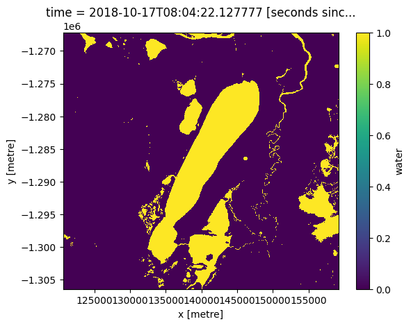
[9]:
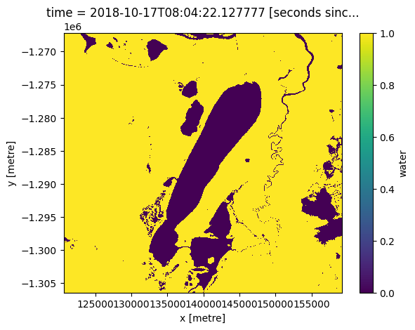
# Show areas flagged as water only (with no other flags set)
(wofl.water == 128).plot.imshow();
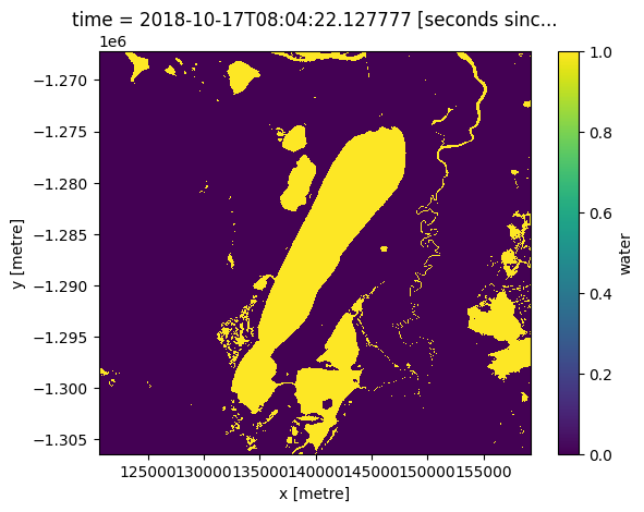
Masking
We can convert the WOFL bit field into a binary array containing True and False values. This allows us to use the WOFL data as a mask that can be applied to other datasets.
The make_mask function allows us to create a mask using the flag labels (e.g. “wet” or “dry”) rather than the binary numbers we used above.
[10]:
# Create a mask based on all 'wet' pixels
wetwofl = masking.make_mask(wofl, wet=True)
wetwofl.water.plot();
Create custom masks by combining flags
Flags can be combined. When chaining flags together, they will be combined in a logical AND fashion. This process works by passing a dictionary with true/false values to the make_mask function. This allows you to chose whether you want to remove clouds and/or cloud shadows from imagery.
[11]:
# Clear (no clouds and shadow)
clear = {"cloud_shadow": False, "cloud": False}

cloudfree = masking.make_mask(wofl, **clear)
cloudfree.water.plot();
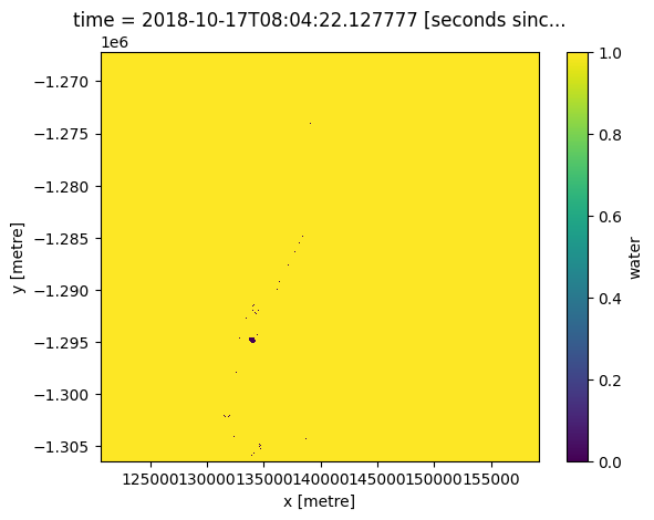
Or, to look at only the clear areas which are good quality data and not wet, we can use the ‘dry’ flag.
[12]:
# clear and dry mask
good_data_mask = masking.make_mask(wofl, dry=True)
good_data_mask.water.plot();
Additional information
License: The code in this notebook is licensed under the Apache License, Version 2.0. Digital Earth Africa data is licensed under the Creative Commons by Attribution 4.0 license.
Contact: If you need assistance, please post a question on the Open Data Cube Slack channel or on the GIS Stack Exchange using the open-data-cube tag (you can view previously asked questions here). If you would like to report an issue with this notebook, you can file one on
Github.
Compatible datacube version:
[13]:
print(datacube.__version__)
1.8.20
Last Tested:
[14]:
from datetime import datetime
datetime.today().strftime('%Y-%m-%d')
[14]:
'2025-01-15'