Calculating band indices with Spyndex package
Products used: s2_l2a
Keywords data used; sentinel-2, band index; NDVI, band package; load_ard, band index; EVIpackage; spyndex`
Background
Remote sensing indices are combinations of spectral bands used to highlight features in the data and the underlying landscape. The Spyndex python package provides access to spectral indices from the Awesome Spectral Indices catalogue. This is a standardized, ready to use, curated list of spectral indices. The Spyndex package currently includes 232 optical and radar indices.
One of the benefits of this package is the large number of optical and radar indices available for DE Africa sandbox users to easily calculate a wide range of remote sensing indices that can be used to assist in mapping and monitoring features like vegetation and water consistently through time, or as inputs to machine learning or classification algorithms using Digital Earth Africa’s archive of analysis-ready satellite data.
Description
This notebook demonstrates how to:
Load Digital Earth Africa’s archive of analysis-ready satellite data using
load_ardCalculate a range of vegetation indices using the
spyndexfunctionPlot the results for all the indices
Getting started
To run this analysis, run all the cells in the notebook, starting with the “Load packages” cell.
Load packages
[1]:
# Load the python packages.
%matplotlib inline

import matplotlib.pyplot as plt
import geopandas as gpd

#import spyndex package
import spyndex

import datacube

from deafrica_tools.datahandling import load_ard, mostcommon_crs
from deafrica_tools.plotting import rgb
from deafrica_tools.bandindices import calculate_indices
from odc.geo.geom import Geometry
from deafrica_tools.areaofinterest import define_area
Connect to the datacube
Connect to the datacube database to enable loading Digital Earth Africa data.
[2]:
# Connect to the datacube
dc = datacube.Datacube(app="spyndex_function")
Select location
Using the define_area function, select area of interest by specifying lat,lon and buffer. If you have the vector or shapefile uncomment the code below Method 2 and replace the aoi.shp with the path of your shapefile.
[3]:
# Method 1: Specify the latitude, longitude, and buffer
aoi = define_area(lat=31.23394, lon=31.05560, buffer=0.02)

# Method 2: Use a polygon as a GeoJSON or Esri Shapefile.
#aoi = define_area(vector_path='aoi.shp')

#Create a geopolygon and geodataframe of the area of interest
geopolygon = Geometry(aoi["features"][0]["geometry"], crs="epsg:4326")
geopolygon_gdf = gpd.GeoDataFrame(geometry=[geopolygon], crs=geopolygon.crs)

# Get the latitude and longitude range of the geopolygon
lat_range = (geopolygon_gdf.total_bounds[1], geopolygon_gdf.total_bounds[3])
lon_range = (geopolygon_gdf.total_bounds[0], geopolygon_gdf.total_bounds[2])
Create a query and load satellite data
To demonstrate how to compute a remote sensing index, we first need to load time series of satellite data for an area. Sentinel-2 satellite data will be used:
It is highly recommended to load data with load_ard when calculating indices. This is because load_ard performs the necessary data cleaning and scaling for more robust index results. Refer to Using_load_ard to learn more
[4]:
# time_range.
time_range = ("2019-06", "2020-06")


# Create a reusable query object.
query = {
    "x": lon_range,
    "y": lat_range,
    "time": time_range,
    "resolution": (-10, 10)
}

# Identify the most common projection system in the input query
output_crs = mostcommon_crs(dc=dc, product="s2_l2a", query=query)

# Load available data from Sentinel-2 and filter to retain only times
# with at least 99% good data
ds = load_ard(
    dc=dc,
    products=["s2_l2a"],
    min_gooddata=0.99,
    measurements=["red", "green", "blue", "nir"],
    output_crs=output_crs,
    **query
)
Using pixel quality parameters for Sentinel 2
Finding datasets
    s2_l2a
Counting good quality pixels for each time step
/opt/venv/lib/python3.12/site-packages/rasterio/warp.py:387: NotGeoreferencedWarning: Dataset has no geotransform, gcps, or rpcs. The identity matrix will be returned.
  dest = _reproject(
Filtering to 78 out of 158 time steps with at least 99.0% good quality pixels
Applying pixel quality/cloud mask
Loading 78 time steps
Selecting a time slide
[5]:
ds = ds.isel(time=[4, 11, 15, 23])
#### Print the xarray dataset
[6]:
print(ds)
<xarray.Dataset> Size: 11MB
Dimensions:      (time: 4, y: 451, x: 390)
Coordinates:
  * time         (time) datetime64[ns] 32B 2019-06-21T08:51:41 ... 2019-09-11...
  * y            (y) float64 4kB 3.459e+06 3.459e+06 ... 3.455e+06 3.455e+06
  * x            (x) float64 3kB 3.129e+05 3.129e+05 ... 3.167e+05 3.168e+05
    spatial_ref  int32 4B 32636
Data variables:
    red          (time, y, x) float32 3MB 530.0 527.0 538.0 ... nan nan nan
    green        (time, y, x) float32 3MB 550.0 533.0 526.0 ... nan nan nan
    blue         (time, y, x) float32 3MB 326.0 344.0 338.0 ... nan nan nan
    nir          (time, y, x) float32 3MB 1.142e+03 1.112e+03 ... nan nan
Attributes:
    crs:           epsg:32636
    grid_mapping:  spatial_ref
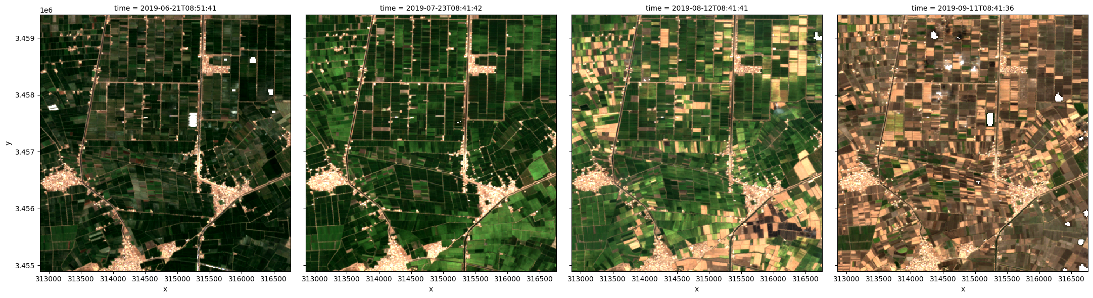
Plot the images in true colour
The rgb function is used to plot the timesteps in our dataset as true colour RGB images:
[7]:
rgb(ds, col='time')
Viewing the attributes for an index
spyndex.indices[indexName] provides the specifications for the index of interest. The cell below prints out the information for the NDVI
[8]:
print(spyndex.indices["NDVI"])
NDVI: Normalized Difference Vegetation Index
        * Application Domain: vegetation
        * Bands/Parameters: ['N', 'R']
        * Formula: (N-R)/(N+R)
        * Reference: https://ntrs.nasa.gov/citations/19740022614
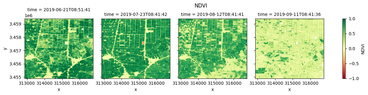
Calculate the Normalized Difference Vegetation Index using the spectral computeIndex method.
The cell below shows how spyndex computes the spectral indices using spectral computeindex function. The spectral computeindex function takes the
indexargument and it specifies the spectral indices that is to be calculatedparamsargument takes the bands from the DE Africa dataset and its corresponding formula name shown in theprint(spyndex.indices["NDVI"])above.NDVINDVI requiresNandRbands as input which are defined for the DE Africa dataset asds.nirandds.red.
[9]:
ds["NDVI"] = spyndex.computeIndex(
    index=["NDVI"],
    params={
        "N": ds.nir,
        "R": ds.red
    }
)
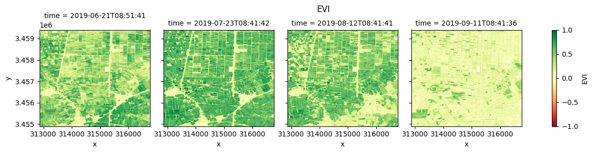
Calculate Enhanced Vegetation Index using spyndex
Using spyndex.indices[indexName] gives the details of the Spectral Index being used. The cell below prints information concerning the EVI Spectral Index.
[10]:
print(spyndex.indices["EVI"])
EVI: Enhanced Vegetation Index
        * Application Domain: vegetation
        * Bands/Parameters: ['g', 'N', 'R', 'C1', 'C2', 'B', 'L']
        * Formula: g*(N-R)/(N+C1*R-C2*B+L)
        * Reference: https://doi.org/10.1016/S0034-4257(96)00112-5
Calculate the Enhanced Vegetation Index index using the spectral computeIndex method.
The EVI has constant values for its computation, as we can see in the formula above.
The Spyndex package provides default constant values which can also be overwritten. The constants can be accessed using spyndex.constants as shown below.
[11]:
ds["EVI"] = spyndex.computeIndex(
    index=["EVI"],
    params={
        "C1": spyndex.constants["C1"].value,
        "C2": spyndex.constants["C2"].value,
        "g": spyndex.constants["g"].value,
        "L": spyndex.constants["L"].value,
        "N": ds.nir,
        "R": ds.red,
        "B": ds.blue,
    },
)
Normalisation
The calculate_indices function from deafrica_tools normalises Sentinel-2 values according to a maximum surface reflectance value of 10,000. We can adapt the Spyndex calculation, as below, to match this normalisation procedure.
[12]:
ds["EVI"] = spyndex.computeIndex(
    index=["EVI"],
    params={
        "C1": spyndex.constants["C1"].value,
        "C2": spyndex.constants["C2"].value,
        "g": spyndex.constants["g"].value,
        "L": spyndex.constants["L"].value,
        "N": ds.nir/10000,
        "R": ds.red/10000,
        "B": ds.blue/10000,
    },
)
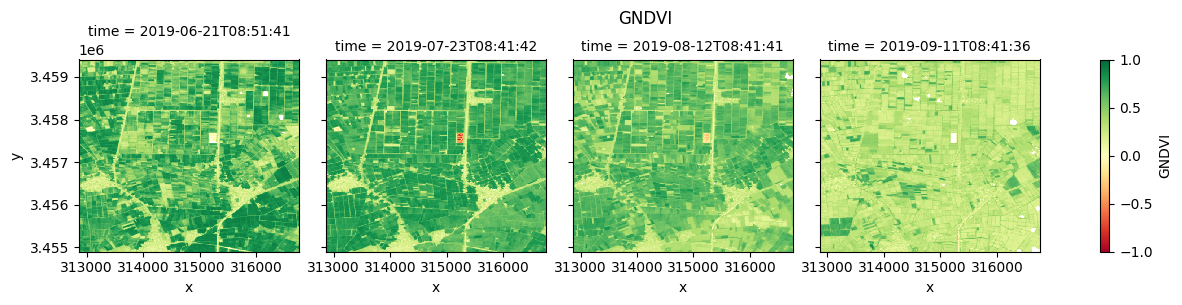
Green Normalized Difference Vegetation Index (GNDVI)
The Green Normalized Difference Vegetation Index GNDVI is a vegetation index for estimating photosynthetic activity and is a commonly used to determine water and nitrogen uptake into the plant canopy. GNDVI is more sensitive to chlorophyll variation in the crop and has a higher saturation point than NDVI. It can be used in crops with dense canopies or in more advanced stages of development. More information can be found in the Reference in the cell below.
Viewing the attributes of the Green Normalized Difference Vegetation Index
[13]:
print(spyndex.indices["GNDVI"])
GNDVI: Green Normalized Difference Vegetation Index
        * Application Domain: vegetation
        * Bands/Parameters: ['N', 'G']
        * Formula: (N-G)/(N+G)
        * Reference: https://doi.org/10.1016/S0034-4257(96)00072-7
Calculate Green Normalized Difference Vegetation Index using spyndex
[14]:
ds["GNDVI"] = spyndex.computeIndex(
    index=["GNDVI"],
    params={
        "N": ds.nir,
        "G": ds.green
    }
)
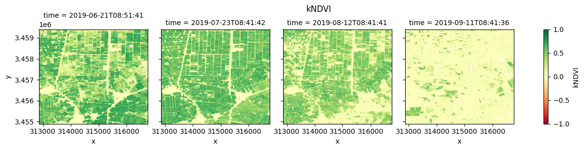
Kernel Normalized Difference Vegetation Index (kNDVI)
The NDVI can only capture linear relationships of the near infrared (NIR) - red difference and a parameter of interest, such as green biomass. In reality, this relationship is nonlinear. Kernel NDVI (kNDVI) was developed to account for higher-order relations between the spectral channels with a nonlinear generalization of the commonly used Normalized Difference Vegetation Index (NDVI). kNDVI has been shown to produce more accurate estimates of key physical variables such as gross primary productivity.
[15]:
print(spyndex.indices["kNDVI"])
kNDVI: Kernel Normalized Difference Vegetation Index
        * Application Domain: kernel
        * Bands/Parameters: ['kNN', 'kNR']
        * Formula: (kNN-kNR)/(kNN+kNR)
        * Reference: https://doi.org/10.1126/sciadv.abc7447
[16]:
# Use the computeKernel() method to compute the required kernel for kernel indices like the kNDVI
# Kernel Normalized Difference Vegetation Index
parameters = {
    "kNN": 1.0,
    "kNR": spyndex.computeKernel(
        kernel="RBF",
        params={"a": ds.nir , "b": ds.red, "sigma": 0.5 * (ds.nir + ds.red)},
    ),
}
ds["kNDVI"] = spyndex.computeIndex("kNDVI", parameters)
Plot each vegetation index
The plot below enables comparison of NDVI, EVI, GNDVI, and kNDVI. Can you observe any differences between the indices? For example, there appears to be more saturation (greater frequency of higher/greener values) for NDVI and GNDVI in the July timestep compared with EVI and kNDVI.
[17]:
#NDVI
fig_ndvi = ds.NDVI.clip(-1,1).plot(col="time", cmap="RdYlGn", vmin=-1, vmax=1)
fig_ndvi.fig.suptitle("NDVI", y= 1.0)
#EVI
fig_evi = ds.EVI.clip(-1,1).plot(col="time", cmap="RdYlGn", vmin=-1, vmax=1)
fig_evi.fig.suptitle("EVI", y= 1.0);
#GNDVI
fig_gndvi = ds.GNDVI.clip(-1,1).plot(col="time", cmap="RdYlGn", vmin=-1, vmax=1)
fig_gndvi.fig.suptitle("GNDVI", y= 1.0)
#kNDVI
fig_kndvi = ds.kNDVI.clip(-1,1).plot(col="time", cmap="RdYlGn", vmin=-1, vmax=1)
fig_kndvi.fig.suptitle("kNDVI", y= 1.0)
plt.show()
Conclusion
This notebook demonstrates how the Spyndex package can be used with DE Africa datasets to compute Spectral Indices. There are 232 optical and radar indices available through the package, try it out and modify the notebook to test different indices and their results.
Additional information
License: The code in this notebook is licensed under the Apache License, Version 2.0. Digital Earth Africa data is licensed under the Creative Commons by Attribution 4.0 license.
Contact: If you need assistance, please post a question on the Open Data Cube Slack channel or on the GIS Stack Exchange using the open-data-cube tag (you can view previously asked questions here). If you would like to report an issue with this notebook, you can file one on
Github.
Compatible datacube version:
[18]:
print(datacube.__version__)
1.8.20
Last Tested:
[19]:
from datetime import date
print(date.today())
2025-01-15