Exporting Cloud-Optimised GeoTIFFs

• Products used: s2_l2a

Keywords data used; sentinel-2, data methods; exporting, data format; GeoTIFF

Background

At the end of an analysis it can be useful to export data to a GeoTIFF file (e.g. outputname.tif), either to save results or to allow for exploring results in a GIS software platform (e.g. ArcGIS or QGIS).

A Cloud Optimized GeoTIFF (COG) is a regular GeoTIFF file, aimed at being hosted on a HTTP file server, with an internal organization that enables more efficient workflows on the cloud.

Description

This notebook shows a number of ways to export a GeoTIFF file:

1. Exporting a single-band, single time-slice GeoTIFF from an xarray object loaded through a dc.load query

2. Exporting a multi-band, single time-slice GeoTIFF from an xarray object loaded through a dc.load query

3. Exporting multiple GeoTIFFs, one for each time-slice of an xarray object loaded through a dc.load query

4. Exporting data from lazily loaded dask arrays

---

Getting started

To run this analysis, run all the cells in the notebook, starting with the “Load packages” cell.

Load packages

%matplotlib inline

import datacube
import geopandas as gpd
from datacube.utils.cog import write_cog
from datacube.utils.geometry import Geometry

from deafrica_tools.datahandling import load_ard
from deafrica_tools.plotting import rgb
from deafrica_tools.areaofinterest import define_area

Connect to the datacube

dc = datacube.Datacube(app='Exporting_GeoTIFFs')

Load Sentinel-2 data from the datacube

Here we are loading in a timeseries of Sentinel-2 satellite images through the datacube API. This will provide us with some data to work with.

The following cell sets the parameters, which define the area of interest and the length of time to conduct the analysis over. The parameters are

• lat: The central latitude to analyse (e.g. 6.502).

• lon: The central longitude to analyse (e.g. -1.409).

• buffer: The number of square degrees to load around the central latitude and longitude. For reasonable loading times, set this as 0.1 or lower.

To define the area of interest, there are two methods available:

1. By specifying the latitude, longitude, and buffer. This method requires you to input the central latitude, central longitude, and the buffer value in square degrees around the center point you want to analyze. For example, lat = 10.338, lon = -1.055, and buffer = 0.1 will select an area with a radius of 0.1 square degrees around the point with coordinates (10.338, -1.055).

2. By uploading a polygon as a GeoJSON or Esri Shapefile. If you choose this option, you will need to upload the geojson or ESRI shapefile into the Sandbox using Upload Files button in the top left corner of the Jupyter Notebook interface. ESRI shapefiles must be uploaded with all the related files (.cpg, .dbf, .shp, .shx). Once uploaded, you can use the shapefile or geojson to define the area of interest. Remember to update the code to call the file you have uploaded.

To use one of these methods, you can uncomment the relevant line of code and comment out the other one. To comment out a line, add the "#" symbol before the code you want to comment out. By default, the first option which defines the location using latitude, longitude, and buffer is being used.

# Set the area of interest

# Method 1: Specify the latitude, longitude, and buffer
aoi = define_area(lat=13.94, lon=-16.54, buffer=0.05)

# Method 2: Use a polygon as a GeoJSON or Esri Shapefile.
# aoi = define_area(vector_path='aoi.shp')

#Create a geopolygon and geodataframe of the area of interest
geopolygon = Geometry(aoi["features"][0]["geometry"], crs="epsg:4326")
geopolygon_gdf = gpd.GeoDataFrame(geometry=[geopolygon], crs=geopolygon.crs)

# Get the latitude and longitude range of the geopolygon
lat_range = (geopolygon_gdf.total_bounds[1], geopolygon_gdf.total_bounds[3])
lon_range = (geopolygon_gdf.total_bounds[0], geopolygon_gdf.total_bounds[2])

# Create a reusable query
query = {
    'x': lon_range,
    'y': lat_range,
    'time': ('2020-11-01', '2020-12-15'),
    'resolution': (-20, 20),
    'measurements': ['red', 'green', 'blue'],
    'output_crs':'EPSG:6933'
}

# Load available data from Landsat 8 and filter to retain only times
# with at least 50% good data
ds = load_ard(dc=dc,
              products=['s2_l2a'],
              **query)

# Print output data
print(ds)

Using pixel quality parameters for Sentinel 2
Finding datasets
    s2_l2a
Applying pixel quality/cloud mask
Loading 9 time steps

/usr/local/lib/python3.10/dist-packages/rasterio/warp.py:344: NotGeoreferencedWarning: Dataset has no geotransform, gcps, or rpcs. The identity matrix will be returned.
  _reproject(

<xarray.Dataset>
Dimensions:      (time: 9, y: 620, x: 483)
Coordinates:
  * time         (time) datetime64[ns] 2020-11-03T11:47:42 ... 2020-12-13T11:...
  * y            (y) float64 1.768e+06 1.768e+06 ... 1.755e+06 1.755e+06
  * x            (x) float64 -1.601e+06 -1.601e+06 ... -1.591e+06 -1.591e+06
    spatial_ref  int32 6933
Data variables:
    red          (time, y, x) float32 nan nan nan nan ... 110.0 131.0 140.0
    green        (time, y, x) float32 nan nan nan nan ... 247.0 248.0 290.0
    blue         (time, y, x) float32 nan nan nan nan ... 99.0 67.0 87.0 89.0
Attributes:
    crs:           EPSG:6933
    grid_mapping:  spatial_ref

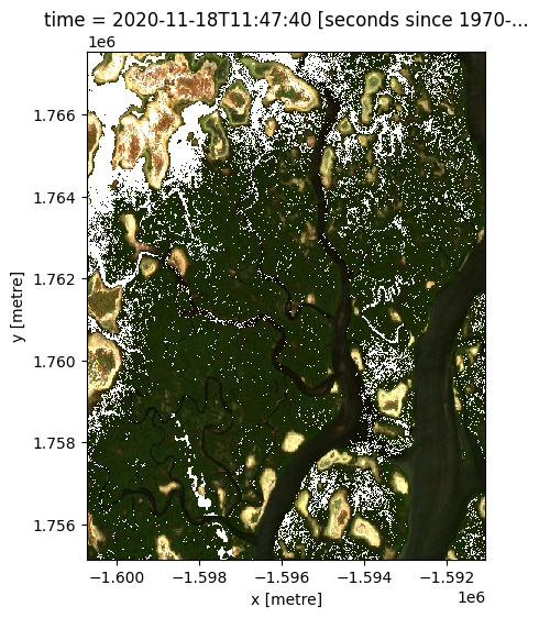
Plot an rgb image to confirm we have data

The white regions are cloud cover.

rgb(ds, index=3)

Export a single-band, single time-slice GeoTIFF

This method uses the datacube.utils.cog function write_cog, where cog stands for Cloud-Optimised-Geotiff to export a simple single-band, single time-slice COG.

A few important caveats should be noted when using this function: 1. It requires an xarray.DataArray; supplying an xarray.Dataset will return an error. To convert a xarray.Dataset to an array run the following:

da = ds.to_array()

2. This function generates a temporary in-memory tiff file without compression. This means the function will use about 1.5 to 2 times the memory required using the depreciated datacube.helper.write_geotiff.

3. If you pass a dask array into the function, write_cog will not output a geotiff, but will instead return aDask Delayed object. To trigger the output of the geotiff run .compute() on the dask delayed object:

   write_cog(ds.red.isel(time=0), "red.tif").compute()
   

# Select a single time-slice and a single band from the dataset.
singleBandtiff = ds.red.isel(time=5)

# Write GeoTIFF to a location
write_cog(singleBandtiff,
          fname="red_band.tif",
          overwrite=True)

PosixPath('red_band.tif')

Export a multi-band, single time-slice GeoTIFF

Here we select a single time and export all the bands in the dataset using the datacube.utils.cog.write_cog function.

# Select a single time-slice
rgb_tiff = ds.isel(time=5).to_array()

# Write multi-band GeoTIFF to a location
write_cog(rgb_tiff,
          fname='rgb.tif',
          overwrite=True)

PosixPath('rgb.tif')

Export multiple GeoTIFFs, one for each time-slice of an xarray

If we want to export all of the time steps in a dataset as a GeoTIFF, we can wrap our write_cog function in a for-loop.

for i in range(len(ds.time)):

    # We will use the date of the satellite image to name the GeoTIFF
    date = ds.isel(time=i).time.dt.strftime('%Y-%m-%d').data
    print(f'Writing {date}')

    # Convert current time step into a `xarray.DataArray`
    singleTimestamp = ds.isel(time=i).to_array()

    # Write GeoTIFF
    write_cog(singleTimestamp,
              fname=f'{date}.tif',
              overwrite=True)

Writing 2020-11-03
Writing 2020-11-08
Writing 2020-11-13
Writing 2020-11-18
Writing 2020-11-23
Writing 2020-11-28
Writing 2020-12-03
Writing 2020-12-08
Writing 2020-12-13

Advanced

Exporting GeoTIFFs from a dask array

If you pass a lazily-loaded dask array into the function, write_cog will not immediately output a GeoTIFF, but will instead return a dask.delayed object:

# Lazily load data using dask
ds_dask = dc.load(product='s2_l2a',
                  dask_chunks={},
                  **query)

# Run `write_cog`
ds_delayed = write_cog(geo_im=ds_dask.isel(time=5).to_array(),
                       fname='dask_geotiff.tif',
                       overwrite=True)

# Print dask.delayed object
print(ds_delayed)

Delayed('_write_cog-5ff4ca46-32b4-44c9-9529-5cfea7c9b1a3')

To trigger the GeoTIFF to be exported to file, run .compute() on the dask.delayed object. The file will now appear in the file browser to the left.

ds_delayed.compute()

PosixPath('dask_geotiff.tif')

---

Additional information

License: The code in this notebook is licensed under the Apache License, Version 2.0. Digital Earth Africa data is licensed under the Creative Commons by Attribution 4.0 license.

Contact: If you need assistance, please post a question on the Open Data Cube Slack channel or on the GIS Stack Exchange using the open-data-cube tag (you can view previously asked questions here). If you would like to report an issue with this notebook, you can file one on Github.

Compatible datacube version:

print(datacube.__version__)

1.8.15

Last Tested:

from datetime import datetime
datetime.today().strftime('%Y-%m-%d')

'2023-08-14'