Land Use Land Cover Maps

• Products used: io_lulc, esa_worldcover_2020, esa_worldcover_2021, cgls_landcover, cci_landcover

Keywords: data used; ESRI Land Cover, datasets; io_lulc, data used; ESA WorldCover, datasets; esa_worldcover_2020 data used; Copernicus Global Land Service, Land Use/Land Cover at 100 m, datasets; cgls_landcover data used; ESA Climate Change Initiative Land Cover, datasets; cci_landcover

Background

Land Use/Land Cover (LULC) maps classify land into broad categories such as water, crops, or built area. They are useful for visualising the dominant land uses in a given area. The total area or proportion of different classes can also be calculated for a specified area.

Many organisations publish LULC maps. DE Africa provides access to the Environmental Systems Research Institute (Esri)/Impact Observatory (IO) land use/land cover (LULC), European Space Agency (ESA) WorldCover, Copernicus Global Land Service (CGLS) Land Use/Land Cover at 100 m, and ESA Climate Change Initiative (CCI) land cover. The ESRI/IO and ESA products are derived from ESA Sentinel imagery and are available at 10 m resolution annually from 2017, 2020 and 2021 respectively over the entire African continent. The CGLS product is available at 100 m resolution, is updated annually and is currently available from 2015 to 2019. The ESA CCI landcover product is available at 300 resolution, is updated annually and is currently available from 1992 to 2019 .

The accuracy of landcover maps changes with location and class, so its important to understand the quality of the maps. ESRI publishes information on the accuracy of the 2020 (10 class version) LULC product, which is neatly summarised in the confusion matrix located here. The overall accuracy for all classes is 85 %. Keep in mind that the accuracy statistics in the link are for the globe and not specific to Africa.

ESA’s WorldCover product comes with an in-depth report on the quality of the product, which we will not reproduce here. However, the full product validation report can be found using the following link: https://esa-worldcover.org/en/data-access. The overall accuracy of the 2020 product for Africa is 73.6%, and it improved to 76.5% in 2021.

The Copernicus Global Land Cover 100m product has a scientific publication exploring the accuracy of the annual landcover maps. The overall accuracy for Africa is ~80 %.

Important details: * Classes and values

io_lulc value	io_lulc class	esa value	esa class	cgls value	cgls class	cci value	cci class
0	no data	0	no data	0	no data	0	no data
1	water	10	tree cover	20	shrubs	10	cropland, rainfed
2	trees	20	shrubland	30	herbaceous vegetation	11	cropland, rainfed, herbaceous cover
3	not used	30	grassland	40	cultivated and managed vegetation or agriculture	12	cropland, rainfed, tree or shrub cover
4	flooded vegetation	40	cropland	50	urban or built up	20	cropland, irrigated or post-flooding
5	crops	50	built up	60	bare or sparse vegetation	30	mosaic cropland/natural vegetation
6	not used	60	bare/sparse vegetation	70	snow and ice	40	mosaic natural vegetation/cropland
7	built area	70	snow and ice	80	permanent water bodies	50	tree cover, broadleaved, evergreen, closed to open
8	bare ground	80	permanent water bodies	90	herbaceous wetland	60	tree cover, broadleaved, deciduous, closed to open
9	snow/ice	90	herbaceous wetland	100	moss and lichen	61	tree cover, broadleaved, deciduous, closed
10	clouds	95	mangroves	111	closed forest, evergreen needle leaf	62	tree cover, broadleaved, deciduous, open
11	rangeland	100	moss and lichen	112	closed forest, evergreen broad leaf	70	tree cover, needleleaved, evergreen, closed to open
				113	closed forest, deciduous needle leaf	71	tree cover, needleleaved, evergreen, closed
				114	closed forest, deciduous broad leaf	72	tree cover, needleleaved, evergreen, open
				115	closed forest, mixed	80	tree cover, needleleaved, deciduous, closed to open
				116	closed forest, unknown	81	tree cover, needleleaved, deciduous, closed
				121	open forest, evergreen needle leaf	82	tree cover, needleleaved, deciduous, open
				122	open forest, evergreen broad leaf	90	tree cover, mixed leaf type
				123	open forest, deciduous needle leaf	100	mosaic tree and shrub/herbaceous cover
				124	open forest, deciduous broad leaf	110	mosaic herbaceous cover/tree and shrub
				125	open forest, mixed	120	shrubland
				126	open forest, unknown	121	shrubland, evergreen
				200	open sea	122	shrubland, deciduous
						130	grassland
						140	lichens and mosses
						150	sparse vegetation
						151	sparse tree
						152	sparse shrub
						153	sparse herbaceous cover
						160	tree cover, flooded, fresh or brakish water
						170	tree cover, flooded, saline water
						180	shrub or herbaceous cover, flooded, fresh/saline/brakish water
						190	urban areas
						200	bare areas
						201	consolidated bare areas
						202	unconsolidated bare areas
						210	water bodies
						220	permanent snow and ice

• Time range and spatial resolution

	io_lulc	esa_worldcover	cgls_landcover	cci_landcover
Time-range	2017-2021	2020-2021	2015-2019	1992-2019
Spatial resolution	10m	10m	100m	300m

Description

In this notebook we will load LULC data using dc.load() to return a map of land use and land cover classes for a specified area.

Topics covered include: 1. Inspecting the LULC product available in the datacube 2. Using the dc.load() function to load in LULC data 3. Plotting LULC using the plot_lulc() function 4. An example analysis of the area of LULC classes in a given area 5. Loading and plotting the ‘cover fractions’ in CGLS

---

Getting started

To run this analysis, run all the cells in the notebook, starting with the “Load packages” cell.

Load packages

%matplotlib inline

import datacube
import numpy as np
import matplotlib.pyplot as plt
import matplotlib.ticker as mticker
from deafrica_tools.plotting import display_map, plot_lulc

Connect to the datacube

dc = datacube.Datacube(app="Landcover_Classification")

List measurements

We can inspect the data available for LULC using datacube’s list_measurements functionality. The table below lists the products and measurements available for the two LULC datasets indexed within DE Africa’s datacube. We can see that the product contains one layer named ‘classification’. The datatype is integer, which corresponds to a LULC class.

product_name = ['io_lulc', 'esa_worldcover_2020', 'esa_worldcover_2021', 'cgls_landcover', 'cci_landcover']

dc_measurements = dc.list_measurements()
dc_measurements.loc[product_name].drop('flags_definition', axis=1)

		name	dtype	units	nodata	aliases
product	measurement
io_lulc	data	data	uint8	1	0.0	[classification]
esa_worldcover_2020	classification	classification	uint8	1	0.0	NaN
esa_worldcover_2021	classification	classification	uint8	1	0.0	NaN
cgls_landcover	classification	classification	uint8	1	255.0	[class]
	forest_type	forest_type	uint8	percent	255.0	[]
	classification_probability	classification_probability	uint8	percent	255.0	[prob]
	bare_cover_fraction	bare_cover_fraction	uint8	percent	255.0	[bare]
	builtup_cover_fraction	builtup_cover_fraction	uint8	percent	255.0	[builtup]
	crops_cover_fraction	crops_cover_fraction	uint8	percent	255.0	[crops]
	grass_cover_fraction	grass_cover_fraction	uint8	percent	255.0	[grass]
	mosslichen_cover_fraction	mosslichen_cover_fraction	uint8	percent	255.0	[mosslichen]
	permanentwater_cover_fraction	permanentwater_cover_fraction	uint8	percent	255.0	[permanentwater]
	seasonalwater_cover_fraction	seasonalwater_cover_fraction	uint8	percent	255.0	[seasonalwater]
	shrub_cover_fraction	shrub_cover_fraction	uint8	percent	255.0	[shrub]
	snow_cover_fraction	snow_cover_fraction	uint8	percent	255.0	[snow]
	tree_cover_fraction	tree_cover_fraction	uint8	percent	255.0	[tree]
cci_landcover	classification	classification	uint8	1	0.0	[class]

Analysis parameters

This section defines the analysis parameters, including:

• lat, lon, buffer: center lat/lon and analysis window size for the area of interest

• resolution: the pixel resolution to use for loading the LULC dataset. The native resolution of the product is 10 metres i.e. (-10,10)

• measurements: the ‘band’ or measurement to load from the product, we can use the native measurement names of one of the aliases

The default location is Madagascar

lat, lon = -19.4557, 46.4644

buffer = 5.0

resolution=(-500, 500) #resample so we can view a large area

measurements='classification'

#convert the lat,lon,buffer into a range
lons = (lon - buffer, lon + buffer)
lats = (lat - buffer, lat + buffer)

Load the LULC datasets

First, we’ll load the ESRI Land Cover. For this annual product, the time window listed in the metadata for a year is from 1 Jan to 1 Jan next year, e.g. 2020 data has a start date of 1 Jan 2020 and end date of 1 Jan 2021. We therefore define the query with both year and month to avoid loading data from a neighboring year.

#create reusable datacube query object
query = {
    'time': ('2020-07'),
    'x': lons,
    'y': lats,
    'resolution':resolution,
    'output_crs': 'epsg:6933',
    'measurements':measurements
}

#load the data
ds_io = dc.load(product='io_lulc', **query).squeeze()

print(ds_io)

<xarray.Dataset>
Dimensions:         (y: 2407, x: 1931)
Coordinates:
    time            datetime64[ns] 2020-07-02
  * y               (y) float64 -1.825e+06 -1.826e+06 ... -3.028e+06 -3.028e+06
  * x               (x) float64 4.001e+06 4.001e+06 ... 4.965e+06 4.966e+06
    spatial_ref     int32 6933
Data variables:
    classification  (y, x) uint8 0 0 0 0 0 0 0 0 0 0 0 ... 0 0 0 0 0 0 0 0 0 0 0
Attributes:
    crs:           epsg:6933
    grid_mapping:  spatial_ref

Now we can load the esa_worldcover_2020,esa_worldcover_2021, cgls_landcover, and cci_landcover products over the same region.

ds_esa_2020 = dc.load(product='esa_worldcover_2020', time='2020', measurements=measurements, like=ds_io.geobox).squeeze()

print(ds_esa_2020)

<xarray.Dataset>
Dimensions:         (y: 2407, x: 1931)
Coordinates:
    time            datetime64[ns] 2020-07-01T12:00:00
  * y               (y) float64 -1.825e+06 -1.826e+06 ... -3.028e+06 -3.028e+06
  * x               (x) float64 4.001e+06 4.001e+06 ... 4.965e+06 4.966e+06
    spatial_ref     int32 6933
Data variables:
    classification  (y, x) uint8 0 0 0 0 0 0 0 0 0 0 0 ... 0 0 0 0 0 0 0 0 0 0 0
Attributes:
    crs:           PROJCS["WGS 84 / NSIDC EASE-Grid 2.0 Global",GEOGCS["WGS 8...
    grid_mapping:  spatial_ref

ds_esa_2021 = dc.load(product='esa_worldcover_2021', time='2021', measurements=measurements, like=ds_io.geobox).squeeze()

print(ds_esa_2021)

<xarray.Dataset>
Dimensions:         (y: 2407, x: 1931)
Coordinates:
    time            datetime64[ns] 2021-07-02
  * y               (y) float64 -1.825e+06 -1.826e+06 ... -3.028e+06 -3.028e+06
  * x               (x) float64 4.001e+06 4.001e+06 ... 4.965e+06 4.966e+06
    spatial_ref     int32 6933
Data variables:
    classification  (y, x) uint8 0 0 0 0 0 0 0 0 0 0 0 ... 0 0 0 0 0 0 0 0 0 0 0
Attributes:
    crs:           PROJCS["WGS 84 / NSIDC EASE-Grid 2.0 Global",GEOGCS["WGS 8...
    grid_mapping:  spatial_ref

ds_cgls = dc.load(product='cgls_landcover', time='2019', measurements=measurements, like=ds_io.geobox).squeeze()

print(ds_cgls)

<xarray.Dataset>
Dimensions:         (y: 2407, x: 1931)
Coordinates:
    time            datetime64[ns] 2019-07-02T11:59:59.500000
  * y               (y) float64 -1.825e+06 -1.826e+06 ... -3.028e+06 -3.028e+06
  * x               (x) float64 4.001e+06 4.001e+06 ... 4.965e+06 4.966e+06
    spatial_ref     int32 6933
Data variables:
    classification  (y, x) uint8 200 200 200 200 200 200 ... 200 200 200 200 200
Attributes:
    crs:           PROJCS["WGS 84 / NSIDC EASE-Grid 2.0 Global",GEOGCS["WGS 8...
    grid_mapping:  spatial_ref

ds_cci = dc.load(product='cci_landcover', time='2019', measurements=measurements, like=ds_io.geobox).squeeze()

print(ds_cci)

<xarray.Dataset>
Dimensions:         (y: 2407, x: 1931)
Coordinates:
    time            datetime64[ns] 2019-07-02T11:59:59.500000
  * y               (y) float64 -1.825e+06 -1.826e+06 ... -3.028e+06 -3.028e+06
  * x               (x) float64 4.001e+06 4.001e+06 ... 4.965e+06 4.966e+06
    spatial_ref     int32 6933
Data variables:
    classification  (y, x) uint8 210 210 210 210 210 210 ... 210 210 210 210 210
Attributes:
    crs:           PROJCS["WGS 84 / NSIDC EASE-Grid 2.0 Global",GEOGCS["WGS 8...
    grid_mapping:  spatial_ref

Plotting data

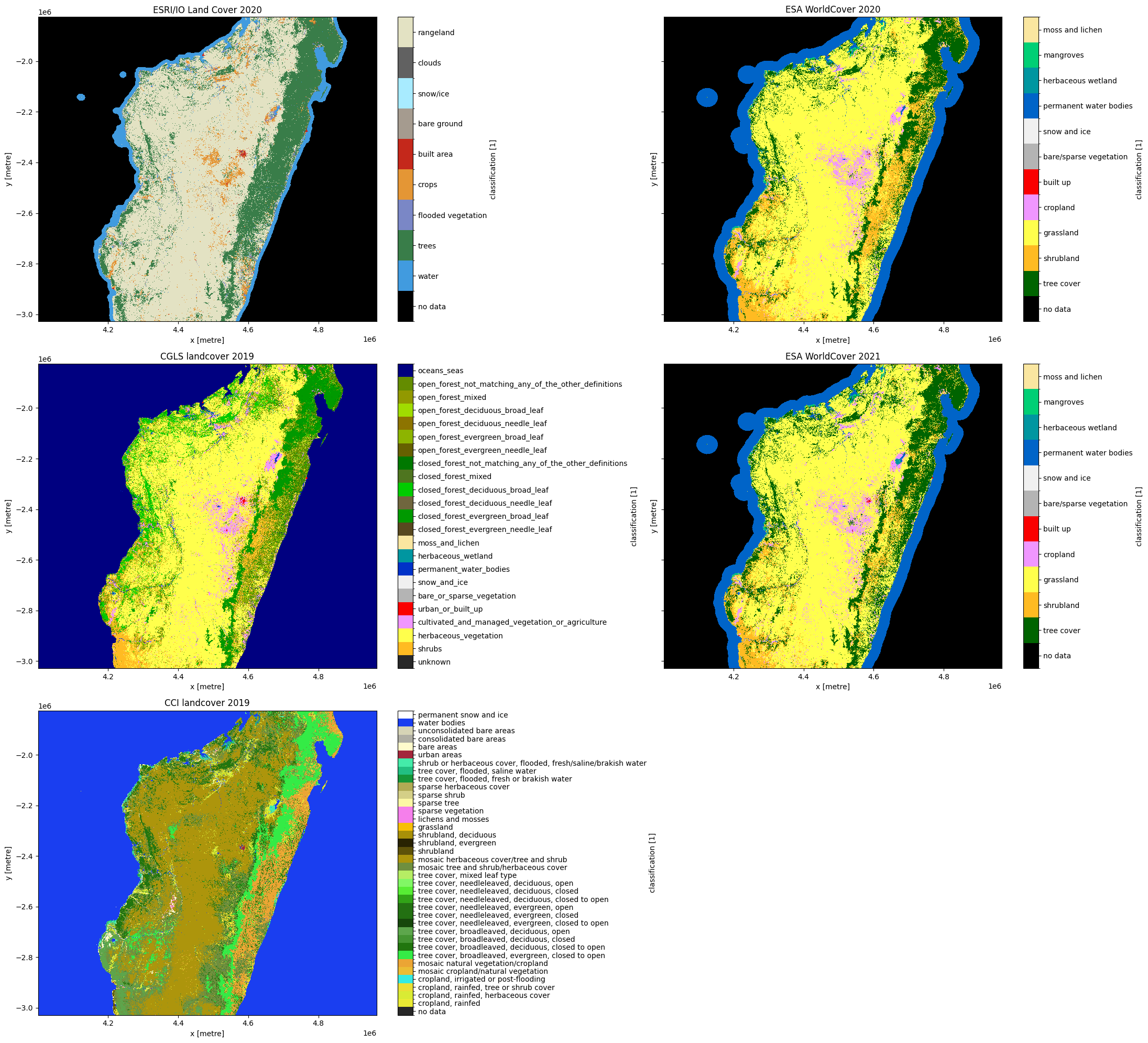
We can plot LULC for Madagascar and add a legend which corresponds to the classes using the DE Africa wrapper function plot_lulc. We can see that trees dominate the eastern areas of the island, while scrub/shrub is more prevalent on the western side. We can also identify a few cities/towns with the red ‘built area’ class. You may also notice that the different datasets don’t always agree.

fig, ax = plt.subplots(3, 2, figsize=(22, 20), sharey=True)
plot_lulc(ds_io[measurements], product="IO", legend=True, ax=ax[0, 0])
plot_lulc(ds_esa_2020[measurements], product="ESA", legend=True, ax=ax[0, 1])
plot_lulc(ds_esa_2021[measurements], product="ESA", legend=True, ax=ax[1, 1])
plot_lulc(ds_cgls[measurements], product="CGLS", legend=True, ax=ax[1, 0])
plot_lulc(ds_cci[measurements], product="CCI", legend=True, ax=ax[2, 0])
ax[0, 0].set_title("ESRI/IO Land Cover 2020")
ax[0, 1].set_title("ESA WorldCover 2020")
ax[1, 1].set_title("ESA WorldCover 2021")
ax[1, 0].set_title("CGLS landcover 2019")
ax[2, 0].set_title("CCI landcover 2019")
fig.delaxes(ax[2, 1])
plt.tight_layout();

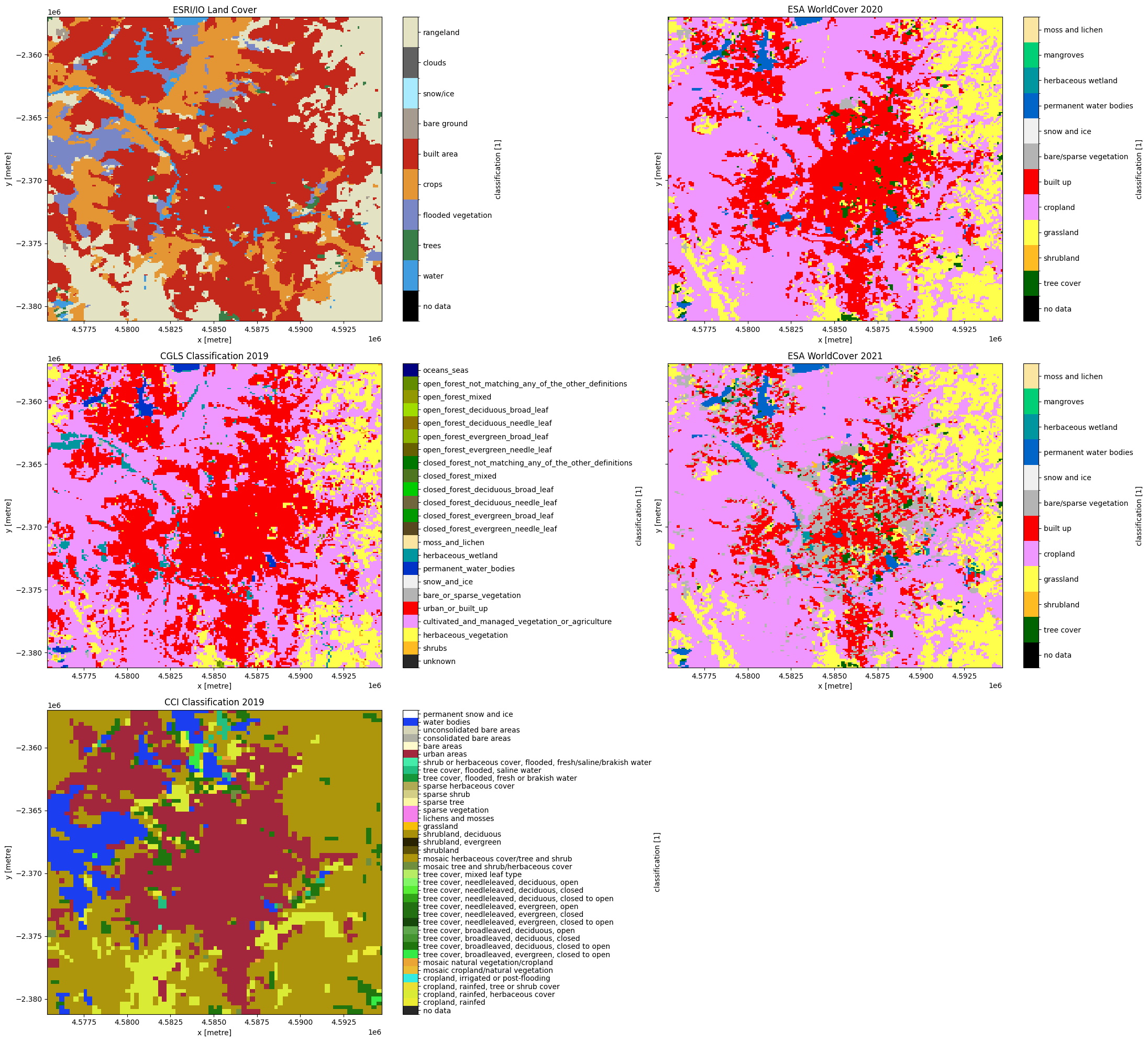
Example Analysis: Investigate the area of classes

In this example, we will look more closely at the city of Antananarivo, the capital of Madagascar, which can be seen in red in the map above. We will load all LULC datasets, calculate the area of each class in each product, and compare the area of classes between the products. As we are looking at a smaller area, we can load the datasets at 100m resolution (its good practice to down-sample higher resolution datasets to a coarser resolution than vice-versa). We use the ‘mode’ statistic to down sample the 10m datasets to 100m resolution, this means each pixel will be assigned the most-common class within the 100m metre pixel.

First, let’s set up some new parameters

lat, lon =  -18.9028, 47.5203
buffer = 0.1
resolution=(-100,100)
measuremnents='classification'

#add lat,lon,buffer to get bounding box
lon_range = (lon-buffer, lon+buffer)
lat_range =  (lat+buffer, lat-buffer)

View selected location

display_map(x=lon_range, y=lat_range)

Make this Notebook Trusted to load map: File -> Trust Notebook

Load LULC data for Antananarivo

query = {
    "x": lon_range,
    "y": lat_range,
    "resolution": resolution,
    "output_crs": "epsg:6933",
    "measurements": measurements,
}

# load the esri product
ds_io = dc.load(product="io_lulc", resampling='mode',
                time='2020-07', **query).squeeze()

# load the esa 2020 product
ds_esa_2020 = dc.load(product="esa_worldcover_2021", resampling='mode',
                 time='2021', measurements=measurements, like=ds_io.geobox).squeeze()

# load the esa 2021 product
ds_esa_2021 = dc.load(product="esa_worldcover_2020", resampling='mode',
                 time='2020', measurements=measurements, like=ds_io.geobox).squeeze()

# load the cgls product
ds_cgls = dc.load(
    product="cgls_landcover",
    time="2019",
    measurements=measurements,
    like=ds_io.geobox
).squeeze()

# load the cci product
ds_cci = dc.load(
    product="cci_landcover",
    time="2019",
    measurements=measurements,
    resampling='nearest',
    like=ds_io.geobox
).squeeze()

Plot the datasets

fig,ax = plt.subplots(3,2, figsize=(22,20), sharey=True)
plot_lulc(ds_io[measurements], product='IO', legend=True, ax=ax[0,0])
plot_lulc(ds_esa_2020[measurements], product='ESA', legend=True, ax=ax[0,1])
plot_lulc(ds_esa_2021[measurements], product='ESA', legend=True, ax=ax[1,1])
plot_lulc(ds_cgls[measurements], product='CGLS', legend=True, ax=ax[1,0])
plot_lulc(ds_cci[measurements], product='CCI', legend=True, ax=ax[2,0])
ax[0,0].set_title('ESRI/IO Land Cover')
ax[0,1].set_title('ESA WorldCover 2020')
ax[1,1].set_title('ESA WorldCover 2021')
ax[1,0].set_title('CGLS Classification 2019')
ax[2,0].set_title('CCI Classification 2019')
fig.delaxes(ax[2, 1])
plt.tight_layout();

Calculate the area of each class

We can use the numpy np.unique function to return the pixel count for each class.

ds_io_counts = np.unique(ds_io[measurements].data, return_counts=True)
ds_esa_2020_counts = np.unique(ds_esa_2020[measurements].data, return_counts=True)
ds_esa_2021_counts = np.unique(ds_esa_2021[measurements].data, return_counts=True)
ds_cgls_counts = np.unique(ds_cgls[measurements].data, return_counts=True)
ds_cci_counts = np.unique(ds_cci[measurements].data, return_counts=True)


print(ds_io_counts)

(array([ 1,  2,  4,  5,  7,  8, 11], dtype=uint8), array([ 1307,   277,  2269,  8079, 23896,   246, 10632]))

We can see above that result is an array with classes 1:11 which corresponds to water through to rangeland, and the count of pixels within these classes. Using the resolution we set in our data loading query, we can calculate the total area of each class in square kilometres and plot the results. Does the plot align with the proportions of classes we can visualise in the map of Antananarivo?

For more information on area calculations see the water extent calculation section of the Digital Earth Africa Sandbox training course.

pixel_length = query["resolution"][1]  # in metres, refers to resolution we defined above (-10,10) for Antananarivo
m_per_km = 1000  # conversion from metres to kilometres
area_per_pixel = pixel_length**2 / m_per_km**2

#calculate the area of each class
ds_io_area = np.array(ds_io_counts[1] * area_per_pixel)
ds_esa_2020_area = np.array(ds_esa_2020_counts[1] * area_per_pixel)
ds_esa_2021_area = np.array(ds_esa_2021_counts[1] * area_per_pixel)
ds_cgls_area = np.array(ds_cgls_counts[1] * area_per_pixel)
ds_cci_area = np.array(ds_cci_counts[1] * area_per_pixel)

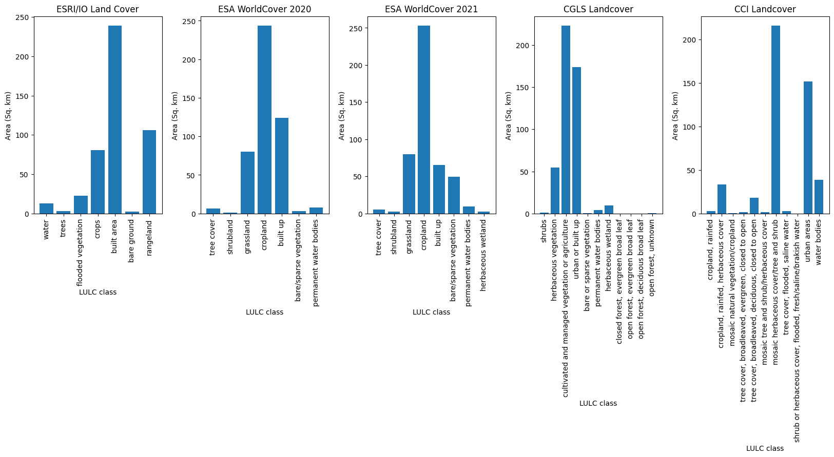
Plot the area of each class

In the plot below, are the proportions of classes similar between the products? What are the classes that typically show confusion?

# list of classes actually in the map by extracting from the `flags_definition`
io_classes = [ds_io.classification.flags_definition['data']['values'][str(x)] for x in ds_io_counts[0]]
esa_classes_2020 = [ds_esa_2020.classification.flags_definition['data']['values'][str(x)] for x in ds_esa_2020_counts[0]]
esa_classes_2021 = [ds_esa_2021.classification.flags_definition['data']['values'][str(x)] for x in ds_esa_2021_counts[0]]
cgls_classes = [ds_cgls.classification.flags_definition['data']['values'][str(x)] for x in ds_cgls_counts[0]]
cci_classes = [ds_cci.classification.flags_definition['data']['values'][str(x)] for x in ds_cci_counts[0]]

fig,ax=plt.subplots(1,5, figsize=(20,5))

#plot esri
ax[0].bar(io_classes, ds_io_area)
ticks_loc = ax[0].get_xticks()
ax[0].xaxis.set_major_locator(mticker.FixedLocator(ticks_loc))
ax[0].set_xticklabels(io_classes, rotation=90)
ax[0].set_xlabel("LULC class")
ax[0].set_ylabel("Area (Sq. km)")

#plot esa worldcover 2020
ax[1].bar(esa_classes_2020, ds_esa_2020_area)
ticks_1 = ax[1].get_xticks()
ax[1].xaxis.set_major_locator(mticker.FixedLocator(ticks_1))
ax[1].set_xticklabels(esa_classes_2020, rotation=90)
ax[1].set_xlabel("LULC class")
ax[1].set_ylabel("Area (Sq. km)")

#plot esa worldcover 2021
ax[2].bar(esa_classes_2021, ds_esa_2021_area)
ticks_1 = ax[2].get_xticks()
ax[2].xaxis.set_major_locator(mticker.FixedLocator(ticks_1))
ax[2].set_xticklabels(esa_classes_2021, rotation=90)
ax[2].set_xlabel("LULC class")
ax[2].set_ylabel("Area (Sq. km)")

#plot cgls
ax[3].bar(cgls_classes, ds_cgls_area)
ticks_2 = ax[3].get_xticks()
ax[3].xaxis.set_major_locator(mticker.FixedLocator(ticks_2))
ax[3].set_xticklabels(cgls_classes, rotation=90)
ax[3].set_xlabel("LULC class")
ax[3].set_ylabel("Area (Sq. km)")

#plot cci
ax[4].bar(cci_classes, ds_cci_area)
ticks_2 = ax[4].get_xticks()
ax[4].xaxis.set_major_locator(mticker.FixedLocator(ticks_2))
ax[4].set_xticklabels(cci_classes, rotation=90)
ax[4].set_xlabel("LULC class")
ax[4].set_ylabel("Area (Sq. km)")

# Adjust spacing between subplots
plt.subplots_adjust(wspace=0.3)

ax[0].set_title('ESRI/IO Land Cover')
ax[1].set_title('ESA WorldCover 2020')
ax[2].set_title('ESA WorldCover 2021')
ax[3].set_title('CGLS Landcover')
ax[4].set_title('CCI Landcover');

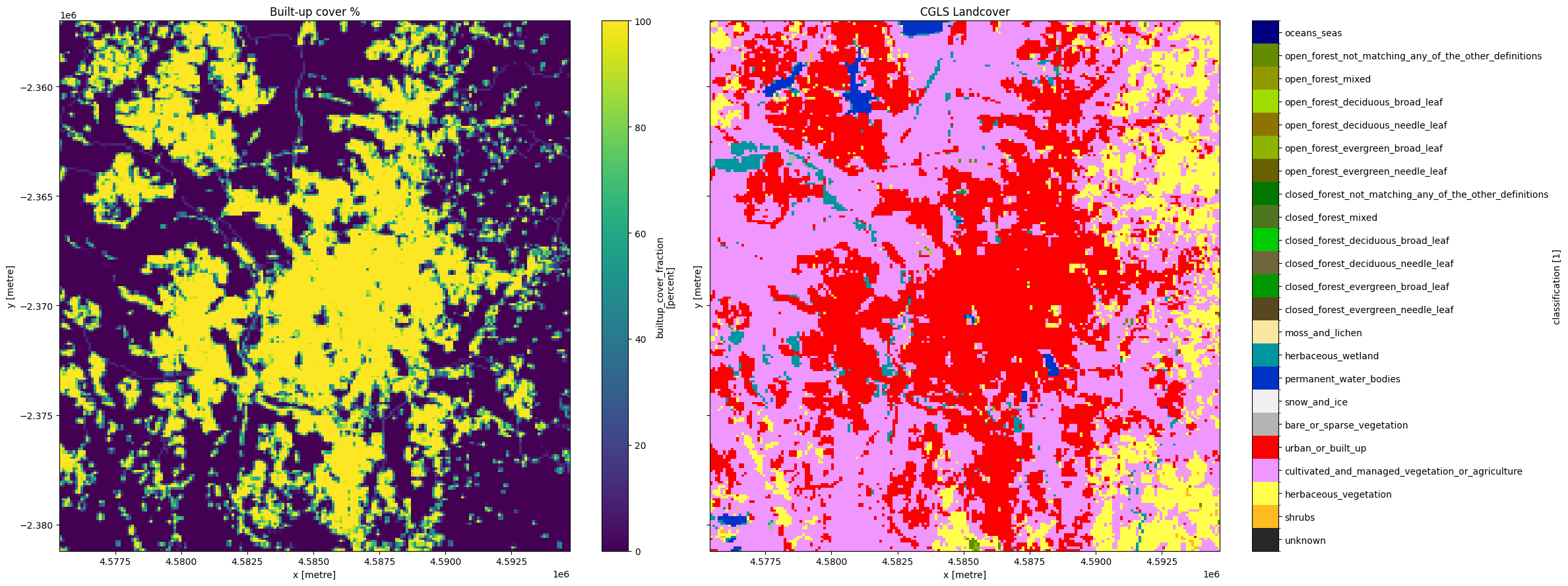
Explore CGLS cover fraction

In the above analysis we can see that the CGLS product classifies a lof of the area in our Antananarivo bounds as ‘urban or built up’. Let’s see how this relates to the builtup cover fraction measurement in the CGLS product.

The cover fraction measurements in CGLS express the percentage of the pixel that is covered by a specific class of land cover, in this case urban or built-up. We can see below that the percentage cover of urban or built-up area corresponds spatially to the landcover classification.

#load the cgls product
ds_cgls_urbancover = dc.load(product='cgls_landcover', time='2019', measurements='builtup_cover_fraction', like=ds_cgls.geobox).squeeze()

#plot the dataset
fig,ax = plt.subplots(1,2, figsize=(24,9), sharey=True)
ds_cgls_urbancover.builtup_cover_fraction.plot(ax=ax[0])
plot_lulc(ds_cgls[measurements], product='CGLS', legend=True, ax=ax[1])

ax[0].set_title('Built-up cover %')
ax[1].set_title('CGLS Landcover')
plt.tight_layout();

---

Additional information

License: The code in this notebook is licensed under the Apache License, Version 2.0. Digital Earth Africa data is licensed under the Creative Commons by Attribution 4.0 license.

Contact: If you need assistance, please post a question on the Open Data Cube Slack channel or on the GIS Stack Exchange using the open-data-cube tag (you can view previously asked questions here). If you would like to report an issue with this notebook, you can file one on Github.

Compatible datacube version:

print(datacube.__version__)

1.8.15

Last tested:

from datetime import datetime
datetime.today().strftime('%Y-%m-%d')

'2023-09-11'