Landsat Surface Temperature 
Keywords data used; landsat 8, data used; landsat 7, data used; landsat 5, datasets; landsat 8, datasets; landsat 7, datasets; landsat 5, surface temperature
Background
The United States Geological Survey’s (USGS) Landsat satellite program has been capturing images of the African continent for more than 30 years. These data are highly useful for land and coastal mapping studies. The Landsat mission not only collects surface reflectance data, but also surface temperature.
Surface temperature measures the Earth’s surface temperature (units of Kelvin) and is an important geophysical parameter in global energy balance studies and hydrologic modeling. Surface temperature is also useful for monitoring crop and vegetation health, and extreme heat events such as natural disasters (e.g. volcanic eruptions, wildfires), and urban heat island effects.
The surface temperature product is generated from:
Landsat Collection 2 Level-1 thermal infrared bands
Top of Atmosphere (TOA) reflectance
TOA brightness temperature
Advanced Spaceborne Thermal Emission and Reflection Radiometer (ASTER) Global Emissivity Database (GED) data
ASTER Normalised Difference Vegetation Index (NDVI) data
Atmospheric profiles of geopotential height, specific humidity, and air temperature extracted from:
Acquisitions 2000 to present: Goddard Earth Observing System (GEOS) Model , Version 5, Forward Processing Instrument Teams (FP-IT)
Acquisitions 1982 to 1999: Modern Era Retrospective analysis for Research and Applications Version 2 (MERRA-2)
For more information and caveats of the product, visit the Landsat Science Products Overview and the Landsat Surface Temperature webpage.
Important details:
Surface temperature product
Native scaling range:
1 - 65,535(0isno-data)To achieve surface temperature values, convert the values to Kelvin using
ds = ds * 0.00341802 + 149.0Using
dc.loadwill load data in the native scaling range1 - 65,535, while usingload_ardwill convert to Kelvin
Native pixel alignment is
centreDate-range: 1984 – present
Spatial resolution: 30 x 30 m
The surface temperature product is provided at 30 m spatial sampling, however, the thermal sensors vary in spectral response, sensitivity and resolution.
For a detailed description of DE Africa’s Landsat archive, see the DE Africa’s Landsat surface temperature technical specifications documentation.
Description
This notebook demonstrates how to load and use the Land Surface Temperature product from the Landsat Collection 2 dataset. Topics covered include:
Load surface temperature and filter with quality assessment
Compare mean surface temperature to daily air temperature at 2-meters height from ERA5
Inspect related land surface characteristics
Getting started
To run this analysis, run all the cells in the notebook, starting with the “Load packages” cell.
Load packages
[1]:
%matplotlib inline

import datacube
import numpy as np
import xarray as xr
import matplotlib.pyplot as plt

from deafrica_tools.load_era5 import load_era5
from deafrica_tools.datahandling import load_ard, mostcommon_crs
from deafrica_tools.plotting import rgb
Connect to the datacube
[2]:
dc = datacube.Datacube(app="Landsat_Surface_Temperature")
Available products and measurements
List products
We can use datacube’s list_products functionality to inspect DE Africa’s Landsat products that are available in the datacube. The table below shows the product names that we will use to load the data, a brief description of the data, and the satellite instrument that acquired the data.
We can search for Landsat Collection 2 Surface Temperature data by using the search term
_st.ststands for “surface temperature”. The datacube is case-sensitive so this must be typed in lower case.
[3]:
# List Landsat products available in DE Africa
dc_products = dc.list_products()
display_columns = ['name', 'description']
dc_products[dc_products.name.str.contains(
    '_st').fillna(
        False)][display_columns].set_index('name')
[3]:
| description | |
|---|---|
| name | |
| ls5_st | USGS Landsat 5 Collection 2 Level-2 Surface Te... |
| ls7_st | USGS Landsat 7 Collection 2 Level-2 Surface Te... |
| ls8_st | USGS Landsat 8 Collection 2 Level-2 Surface Te... |
| ls9_st | USGS Landsat 9 Collection 2 Level-2 Surface Te... |
List measurements
We can further inspect the data available for each Landsat product using datacube’s list_measurements functionality. The table below lists each of the measurements available in the data.
Note that Landsat 8 surface temperature products are generated with a different algorithm from Landsat 5 and 7. It therefore has different output measurements.
[4]:
dc_measurements = dc.list_measurements()
dc_measurements.loc['ls8_st']
[4]:
| name | dtype | units | nodata | aliases | flags_definition | add_offset | scale_factor | |
|---|---|---|---|---|---|---|---|---|
| measurement | ||||||||
| ST_B10 | ST_B10 | uint16 | Kelvin | 0.0 | [band_10, st, surface_temperature] | NaN | NaN | NaN |
| ST_TRAD | ST_TRAD | int16 | W/(m2.sr.μm) | -9999.0 | [trad, thermal_radiance] | NaN | NaN | NaN |
| ST_URAD | ST_URAD | int16 | W/(m2.sr.μm) | -9999.0 | [urad, upwell_radiance] | NaN | NaN | NaN |
| ST_DRAD | ST_DRAD | int16 | W/(m2.sr.μm) | -9999.0 | [drad, downwell_radiance] | NaN | NaN | NaN |
| ST_ATRAN | ST_ATRAN | int16 | 1 | -9999.0 | [atran, atmospheric_transmittance] | NaN | NaN | NaN |
| ST_EMIS | ST_EMIS | int16 | 1 | -9999.0 | [emis, emissivity] | NaN | NaN | NaN |
| ST_EMSD | ST_EMSD | int16 | 1 | -9999.0 | [emsd, emissivity_stddev] | NaN | NaN | NaN |
| ST_CDIST | ST_CDIST | int16 | Kilometers | -9999.0 | [cdist, cloud_distance] | NaN | NaN | NaN |
| QA_PIXEL | QA_PIXEL | uint16 | bit_index | 1.0 | [pq, pixel_quality] | {'snow': {'bits': 5, 'values': {'0': 'not_high... | NaN | NaN |
| QA_RADSAT | QA_RADSAT | uint16 | bit_index | 0.0 | [radsat, radiometric_saturation] | {'nir_saturation': {'bits': 4, 'values': {'0':... | NaN | NaN |
| ST_QA | ST_QA | int16 | Kelvin | -9999.0 | [st_qa, surface_temperature_quality] | NaN | NaN | NaN |
Load Landsat surface temperature using dc.load()
Now that we know what products and measurements are available for the products, we can load data from the datacube using dc.load.
In the example below, we will load surface temperature data from Landsat 8 for Namibia, across parts of 2018 and 2019. First, we will set up the parameters of our data load: latitude and longitude, time, and band measurements.
By specifying output_crs='EPSG:32633' and resolution=(-30, 30), we request that datacube reproject our data to the desired Coordinate Reference System (CRS), with 30 x 30 m pixels.
Note: For a more general discussion of how to load data using the datacube, refer to the Introduction to loading data notebook.
[5]:
# Define the analysis region (Lat-Lon box)
# High Energy Stereoscopic System site near Windhoek Namibia
lat = (-23.275, -23.265)
lon = (16.495, 16.505)

# Define the time window
time = ('2018-07-01', '2019-05-31')

# Load land surface temperature and quality assessment
# We can use the alias names to call the bands
measurements = ['surface_temperature', 'surface_temperature_quality']
[6]:
data = dc.load(product='ls8_st',
               x=lon,
               y=lat,
               time=time,
               measurements = measurements,
               output_crs = 'EPSG:32633',
               resolution = (-30, 30))

print(data)
<xarray.Dataset> Size: 116kB
Dimensions:                      (time: 21, y: 38, x: 36)
Coordinates:
  * time                         (time) datetime64[ns] 168B 2018-07-14T08:50:...
  * y                            (y) float64 304B -2.574e+06 ... -2.575e+06
  * x                            (x) float64 288B 6.529e+05 ... 6.54e+05
    spatial_ref                  int32 4B 32633
Data variables:
    surface_temperature          (time, y, x) uint16 57kB 37333 37339 ... 44213
    surface_temperature_quality  (time, y, x) int16 57kB 636 636 635 ... 176 172
Attributes:
    crs:           EPSG:32633
    grid_mapping:  spatial_ref
Plotting Landsat data from dc.load
We can plot the data we loaded for each timestep and inspect it.
[7]:
data.surface_temperature.plot.imshow(col='time', col_wrap=10, cmap='coolwarm');
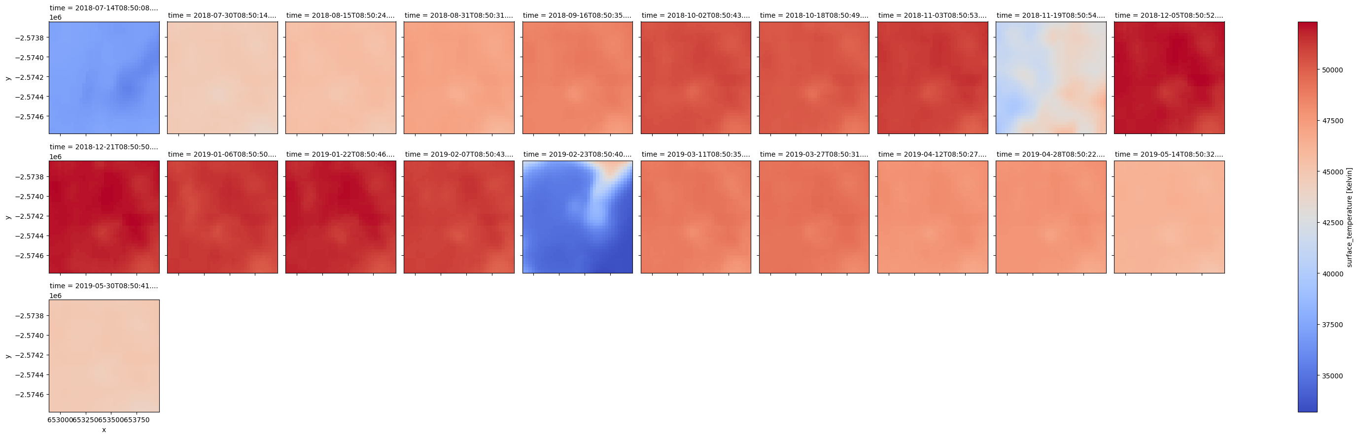
Notice the scale of surface temperature is very large. This is because the data loaded with dc.load has not been scaled according to the scale factor and offsets determined by USGS. Loading data with load_ard performs that scaling automatically, to give temperature in Kelvin.
Load Landsat using load_ard
load_ard applies the linear scaling and offset which converts the native loaded data to actual surface temperature values. load_ard will additionally concatenate and sort the observations by time, and apply a cloud mask. The result is an analysis-ready dataset, which is much easier to use.
In the example below, we load Landsat 8 data for the same time and place as above. We will call this dataset ds to distinguish it from the previously-loaded dataset. Note a cloud mask has now been applied. load_ard also converts the temperature data into Kelvin.
You can find more information on the load_ard function from the Using load ard notebook.
[8]:
ds = load_ard(dc=dc,
               products=['ls8_st'],
               x=lon,
               y=lat,
               time=time,
               measurements = measurements,
               output_crs = 'EPSG:32633',
               resolution = (-30, 30))

print(ds)
Using pixel quality parameters for USGS Collection 2
Finding datasets
    ls8_st
Applying pixel quality/cloud mask
Re-scaling Landsat C2 data
Loading 21 time steps
/opt/venv/lib/python3.12/site-packages/deafrica_tools/datahandling.py:565: FutureWarning: In a future version of xarray the default value for compat will change from compat='no_conflicts' to compat='override'. This is likely to lead to different results when combining overlapping variables with the same name. To opt in to new defaults and get rid of these warnings now use `set_options(use_new_combine_kwarg_defaults=True) or set compat explicitly.
  ds = xr.merge([ds_data, ds_masks])
<xarray.Dataset> Size: 231kB
Dimensions:                      (time: 21, y: 38, x: 36)
Coordinates:
  * time                         (time) datetime64[ns] 168B 2018-07-14T08:50:...
  * y                            (y) float64 304B -2.574e+06 ... -2.575e+06
  * x                            (x) float64 288B 6.529e+05 ... 6.54e+05
    spatial_ref                  int32 4B 32633
Data variables:
    surface_temperature          (time, y, x) float32 115kB nan nan ... 300.1
    surface_temperature_quality  (time, y, x) float32 115kB nan nan ... 1.72
Attributes:
    crs:           EPSG:32633
    grid_mapping:  spatial_ref
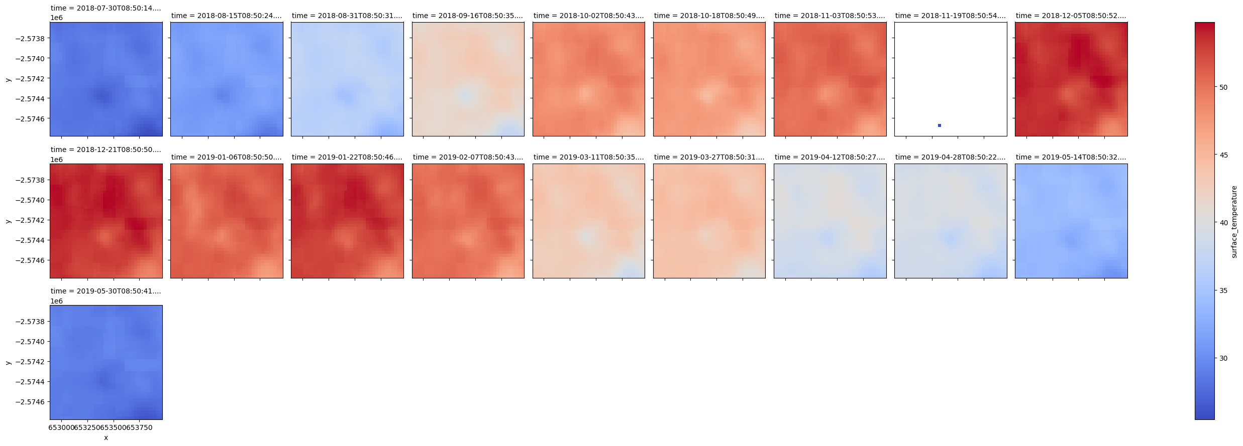
We now want to drop empty slices and convert the surface_temperature band to degrees Celsius. We then plot the time slices with valid data.
[9]:
ds = ds.dropna(dim='time', how='all')
ds['surface_temperature'] = ds.surface_temperature - 273.15
[10]:
ds.surface_temperature.plot.imshow(col='time', col_wrap=9, cmap='coolwarm');
Compare mean surface temperature to daily air temperature
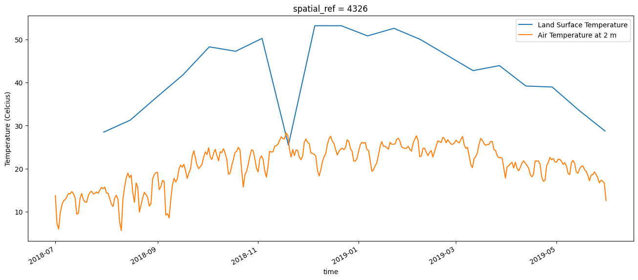
We can load some ERA5 atmospheric data to compare with the Landsat 8 mean surface temperature. Here we use ERA5 daily air temperature at 2 metres height. It is loaded using the load_era5 function and then converted into degrees Celsius. For more information on the ERA5 data and how it is loaded into the Sandbox, see the Climate Data ERA5 notebook.
To plot the data together, we find the average of the land surface temperature over our selected area. This can then be shown together with the corresponding 2-metre air temperature data.
[11]:
# Load ERA5 air temperature at 2 m height
var = 'air_temperature_at_2_metres'

air_temp = load_era5(var, lat, lon, time, reduce_func=np.mean)[var] - 273.15
Opening ERA5 Zarr dataset...
Variable: air_temperature_at_2_metres
Mapped ERA5 name: 2m_temperature
Time: 2018-07-01 to 2019-05-31
Latitude: -23.275 to -23.265
Longitude: 16.495000000000005 to 16.504999999999995
Selecting time range...
Normalising longitude coordinates...
Selecting AOI...
Subset size: {'time': 8040, 'latitude': 1, 'longitude': 1}
Resampling to 1D using <function mean at 0x7f281639b740>...
ERA5 loading complete.
[12]:
ds_mean = ds.groupby('time').mean(dim=xr.ALL_DIMS)
[13]:
ds_mean.surface_temperature.plot(figsize = (16, 6),label='Land Surface Temperature');
air_temp.groupby('time').mean(dim=None).plot(label='Air Temperature at 2 m');
plt.ylabel('Temperature (Celcius)')
plt.legend()
[13]:
<matplotlib.legend.Legend at 0x7f25d0970200>
Additional information
License: The code in this notebook is licensed under the Apache License, Version 2.0. Digital Earth Africa data is licensed under the Creative Commons by Attribution 4.0 license.
Contact: If you need assistance, please post a question on the Open Data Cube Slack channel or on the GIS Stack Exchange using the open-data-cube tag (you can view previously asked questions here). If you would like to report an issue with this notebook, you can file one on
Github.
Compatible datacube version:
[14]:
print(datacube.__version__)
1.9.13
Last Tested:
[15]:
from datetime import datetime
datetime.today().strftime('%Y-%m-%d')
[15]:
'2026-04-30'