Global Mangrove Watch
Products used: gmw
Keywords: :index: ‘data used; Global Mangrove Watch’, :index: ‘datasets; gmw’
Background
The Global Mangrove Watch dataset provides information about mangrove extent. It uses ALOS PALSAR and Landsat (optical) data to form a baseline extent of mangroves. This dataset has been rasterized and indexed from the UN Environment Program into DE Africa’s Open Data Cube. It can also be visualised in the Global Mangrove Extent Explorer.
The dataset can be used to identify mangrove ecosystems and monitor changes in mangrove extent. This is important in applications such as quantifying ‘blue carbon’, mitigating risks from natural disasters, and prioritising restoration activities.
Important details:
This dataset is available in 0.0002 degrees resolution (~ 24 m) for the following years:
1996
2007
2008
2009
2010
2015
2016
2017
2018
2019
2020
Reference
Bunting P., Rosenqvist A., Lucas R., Rebelo L-M., Hilarides L., Thomas N., Hardy A., Itoh T., Shimada M. and Finlayson C.M. (2018). The Global Mangrove Watch – a New 2010 Global Baseline of Mangrove Extent. Remote Sensing 10(10): 1669. doi: 10.3390/rs1010669
Description
In this notebook we will load the Global Mangrove Watch dataset using dc.load(). Then we run through a short comparison of mangrove extent between years.
Topics covered include:
Inspecting the gmw product available in the datacube
Using the
dc.load()function to load in gmw dataPlotting gmw
Getting started
To run this analysis, run all the cells in the notebook, starting with the “Load packages” cell.
Load packages
[1]:
%matplotlib inline

import datacube
import numpy as np
import xarray as xr
import matplotlib.pyplot as plt

from deafrica_tools.plotting import display_map
Connect to the datacube
[2]:
dc = datacube.Datacube(app="gmw")
List measurements
The table below shows that the measurement in the Global Mangrove Watch dataset is called ‘mangrove’, which is a binary classification where 1 corresponds to mangroves and 0 is no mangroves.
[3]:
product_name = ['gmw']

dc_measurements = dc.list_measurements()
dc_measurements.loc[product_name].drop('flags_definition', axis=1)
[3]:
| name | dtype | units | nodata | aliases | ||
|---|---|---|---|---|---|---|
| product | measurement | |||||
| gmw | mangrove | mangrove | uint8 | 1 | 0.0 | [classification] |
Set parameters
lat,lon: The central latitude and longitude to analyse e.g. -16.2818, 39.8633 along the coast of Mozambiquebuffer: The number of square degrees to load around the central latitude and longitude. For quick loading times, set this as 0.1 or lower.resolution: We use 20 m here, as it is closest to the native resolution of 0.0002 degrees.
[4]:
lat, lon =  -16.2818, 39.8633 #along the coast of Mozambique
buffer = 0.15

resolution=(-20, 20)

measurements='mangrove'

#convert the lat,lon,buffer into a range
lons = (lon - buffer, lon + buffer)
lats = (lat - buffer, lat + buffer)
View the selected location
The next cell will display the selected area on an interactive map. Feel free to zoom in and out to get a better understanding of the area you’ll be analysing. Clicking on any point of the map will reveal the latitude and longitude coordinates of that point.
[5]:
display_map(x=lons, y=lats)
[5]:
Load the Global Mangrove Watch data
[6]:
#set up datacube query object
query = {
    'x': lons,
    'y': lats,
    'resolution':resolution,
    'output_crs': 'epsg:6933',
    'measurements':measurements
}

#load the gmw product
ds = dc.load(product="gmw", **query).squeeze()
print(ds)
<xarray.Dataset>
Dimensions:      (time: 11, y: 1839, x: 1448)
Coordinates:
  * time         (time) datetime64[ns] 1996-07-01T23:59:59.500000 ... 2020-07...
  * y            (y) float64 -2.032e+06 -2.032e+06 ... -2.068e+06 -2.068e+06
  * x            (x) float64 3.832e+06 3.832e+06 ... 3.861e+06 3.861e+06
    spatial_ref  int32 6933
Data variables:
    mangrove     (time, y, x) uint8 0 0 0 0 0 0 0 0 0 0 ... 0 0 0 0 0 0 0 0 0 0
Attributes:
    crs:           epsg:6933
    grid_mapping:  spatial_ref
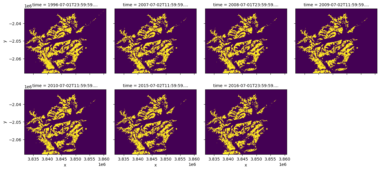
Plot mangrove extent
We can generate a basic plot of mangrove extent for each of the available years below.
[7]:
ds.mangrove.plot(col="time", col_wrap=4, add_colorbar=False);
Analysis example: mangrove area calculation
In this notebook, we conduct a simple calculation of mangrove area as an analysis example. A much more comprehensive and detailed example of mangrove analysis is available in real world examples. The real world example classifies mangroves as ‘closed’ or ‘regular’ and identifies areas of mangrove growth and loss.
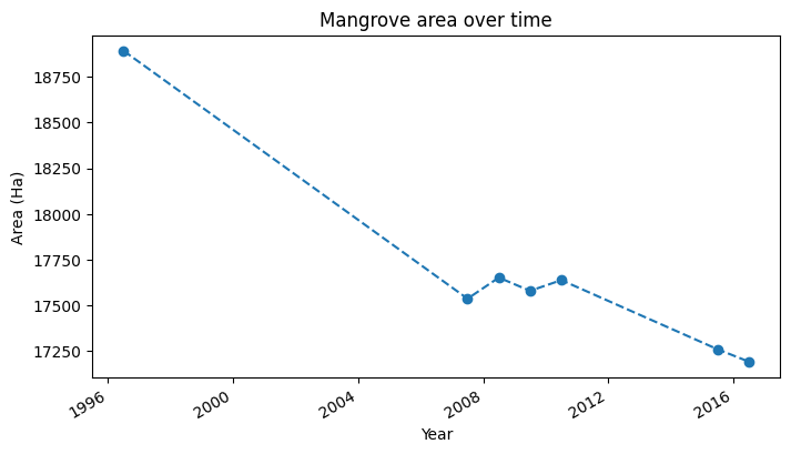
Calculate area
We can calculate the area of mangroves in each of the seven available years, then look for change. In this case ~1,500 Ha of mangrove has disapeared since 1996. Again, the mangrove analysis notebook in real world examples gives a more comprehensive example of assessing changes in mangrove extent.
[8]:
# Convert pixel count to ha
m2_per_ha = 10000
m2_per_pixel = query["resolution"][1] ** 2
mangrove_area = ds.mangrove.sum(dim=("x", "y")) * m2_per_pixel / m2_per_ha

mangrove_area.plot(
    x="time",
    figsize=(8,4),
    linestyle="--",
    marker="o",
)
plt.xlabel("Year")
plt.ylabel("Area (Ha)")
plt.title("Mangrove area over time");
Additional information
License: The code in this notebook is licensed under the Apache License, Version 2.0. Digital Earth Africa data is licensed under the Creative Commons by Attribution 4.0 license.
Contact: If you need assistance, please post a question on the Open Data Cube Slack channel or on the GIS Stack Exchange using the open-data-cube tag (you can view previously asked questions here). If you would like to report an issue with this notebook, you can file one on
Github.
Compatible datacube version:
[9]:
print(datacube.__version__)
1.8.15
Last tested:
[10]:
from datetime import datetime
datetime.today().strftime('%Y-%m-%d')
[10]:
'2024-07-08'