Water Observations from Space (WOfS)
Products used: wofs_ls, wofs_ls_summary_annual, wofs_ls_summary_alltime
Keywords: datasets; wofs_ls, datasets; wofs_ls_summary_alltime, datasets; wofs_ls_summary_annual
Background
Water Observations from Space (WOfS) is a service that draws on satellite imagery to provide historical surface water observations of the whole African continent. WOfS allows users to understand the location and movement of inland and coastal water present in the African landscape. It shows where water is usually present; where it is seldom observed; and where inundation of the surface has been observed by satellite.
They are generated using the WOfS classification algorithm on Landsat satellite data. There are several WOfS products available for the African continent, as listed below:
Product Type |
Description |
|---|---|
WOfS Annual Summary |
The ratio of wet to clear observations from each calendar year |
WOfS All-Time Summary |
The ratio of wet to clear observations over all time |
WOFLs (WOfS Feature Layers) |
Water and non-water classification generated per scene |
WOfS Annual/All-Time Summary: The frequency a pixel was classified as wet. This requires:
Total number of clear observations for each pixel: the number of observations that were clear (no cloud or shadow) for the selected time period. The classification algorithm then assigns these as either wet, or dry.
Total number of wet observation for each pixel: the number of observations that were clear and wet for the selected time period.
The WOfS Summaries are calculated as the ratio of clear wet observations to total clear observations.
WOFLs (WOfS Feature Layers): Individual water-classified images are called Water Observation Feature Layers (WOFLs), and are created from the input satellite data. There is one WOFL for each satellite dataset processed for the occurrence of water. For more information on WOFLs, see the Applying WOfS bitmasking notebook.
Reference
Mueller, N., Lewis, A., Roberts, D., Ring, S., Melrose, R., Sixsmith, J., Lymburner, L., McIntyre, A., Tan, P., Curnow, S., & Ip, A. (2016). Water observations from space: Mapping surface water from 25 years of Landsat imagery across Australia. Remote Sensing of Environment, 174, 341-352.
Description
This notebook explains loading WOFLs and the WOfS summaries.
This notebook demonstrates how to:
Load and plot WOFLS for multiple time-steps
Load WOfS annual summaries
Load the WOfS all-time summary
For a detailed example of using WOfS for water resource management, see the Water_extent_WOfS notebook in the DE Africa sandbox.
Getting Started
To run this analysis, run all the cells in the notebook, starting with the “Load packages” cell.
Load packages
[1]:
%matplotlib inline

import datacube
import seaborn as sns
import matplotlib.pyplot as plt
from datacube.utils import masking
from datacube.utils import geometry
from datacube.utils.geometry import CRS

from deafrica_tools.plotting import display_map, plot_wofs
from deafrica_tools.datahandling import wofs_fuser, mostcommon_crs
Connect to the datacube
[2]:
dc = datacube.Datacube(app="Intro_WOfS")
List of WOfS products available in Digital Earth Africa
[3]:
products = dc.list_products()
display_columns = ['name', 'description']
dc_products = products[display_columns]
dc_products[dc_products['name'].str.contains("wofs_ls")]
[3]:
| name | description | |
|---|---|---|
| name | ||
| wofs_ls | wofs_ls | Historic Flood Mapping Water Observations from... |
| wofs_ls_summary_alltime | wofs_ls_summary_alltime | Water Observations from Space Alltime Statistics |
| wofs_ls_summary_annual | wofs_ls_summary_annual | Water Observations from Space Annual Statistics |
Analysis parameters
The following items are included in the “query” that defines what the datacube need to return.
lat, lon, buffer: center lat/lon and analysis window size for the area of interesttime: date range to fetch the scenes. The approximate time between two scenes is 16 days. If there is a location near a swathe boundary, it may be captured in two passes and so there could be two images within the 16 day period.
The default location is Lake Ngami in Botswana.
[4]:
lat, lon =  -20.4855, 22.7547
buffer = 0.175
time_range = ('2019-01-01', '2019-01-20')

#add lat,lon,buffer togethert to get bounding box
x = (lon-buffer, lon+buffer)
y =  (lat+buffer, lat-buffer)
View the selected location
[5]:
# View the location
display_map(x=x, y=y)
[5]:
Load WOfS Feature Layers (WOFLs)
Here, it is not necessary to directly call on the bit flags as we can use the selection wet=True to create the water mask, while dry=True gives the opposite. In this case, isel is used to select a single timestep, and shows the wet/dry pixels for that increment only.
[6]:
# Create a reusable query
query = {
    'x': x,
    'y': y,
    'time': time_range,
    'resolution': (-30, 30)
}

#grab crs of location
output_crs = mostcommon_crs(dc=dc, product='wofs_ls', query=query)

# Load WOfS feature layers
wofls= dc.load(product = 'wofs_ls',
               group_by="solar_day",
               fuse_func=wofs_fuser,
               output_crs = output_crs,
               collection_category="T1",
               **query)
print(wofls)
<xarray.Dataset>
Dimensions:      (time: 4, y: 1306, x: 1231)
Coordinates:
  * time         (time) datetime64[ns] 2019-01-09T08:26:36.339805 ... 2019-01...
  * y            (y) float64 -2.247e+06 -2.247e+06 ... -2.286e+06 -2.286e+06
  * x            (x) float64 6.646e+05 6.646e+05 ... 7.014e+05 7.015e+05
    spatial_ref  int32 32634
Data variables:
    water        (time, y, x) uint8 64 64 64 64 64 64 64 64 ... 0 0 0 0 0 0 0 0
Attributes:
    crs:           epsg:32634
    grid_mapping:  spatial_ref
Plotting data
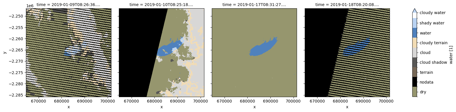
We can plot WOFLs using the plot_wofs function. We can see that our study area includes one large waterbody. We can also see that some observations contain clouds, cloud shadow, and regions of no-data.
[7]:
# Classify different types of data in the area of interest
plot_wofs(wofls.water, col='time', size=4, col_wrap=4);
Masking using WOfS bit flags
WOFLs uses bit flags to flag pixels as “wet” or otherwise. For more details on bitmasking with WOfS, see the Applying WOfS bitmasking notebook.
We can convert the WOfS bit field into a binary array containing True and False values. This allows us to use the WOFL data as a mask that can be applied to other datasets.
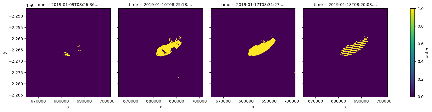
The make_mask function allows us to create a mask using the flag labels (e.g. “wet” or “dry”) rather than the binary numbersin the mask. For example, we can easily identify pixels that were wet in each image (i.e. yellow) by passing the flag wet=True:
[8]:
# Keeping only dry, non-cloudy pixels
wofls_wet = masking.make_mask(wofls, wet=True)

# Plot output mask
wofls_wet.water.plot(col='time', size=4, col_wrap=4);
Loading WOfS annual summaries
To look at a summary of WOFLs over a calender year, we can load the wofs_ls_summary_annual product. This can be useful to understand at a glance the annual dynamics of a waterbody. The WOfS Annual Summary product is pre-calculated, which makes it faster to load. It has three measuremts: count_wet, count_clear, and frequency.
[9]:
wofs_annual = dc.load(product='wofs_ls_summary_annual',
               like=wofls.geobox,
               time='2019')

print(wofs_annual)
<xarray.Dataset>
Dimensions:      (time: 1, y: 1306, x: 1231)
Coordinates:
  * time         (time) datetime64[ns] 2019-07-02T11:59:59.999999
  * y            (y) float64 -2.247e+06 -2.247e+06 ... -2.286e+06 -2.286e+06
  * x            (x) float64 6.646e+05 6.646e+05 ... 7.014e+05 7.015e+05
    spatial_ref  int32 32634
Data variables:
    count_wet    (time, y, x) int16 0 0 0 0 0 0 0 0 0 0 ... 0 0 0 0 0 0 0 0 0 0
    count_clear  (time, y, x) int16 35 34 34 34 34 34 34 ... 51 51 51 51 51 51
    frequency    (time, y, x) float32 0.0 0.0 0.0 0.0 0.0 ... 0.0 0.0 0.0 0.0
Attributes:
    crs:           PROJCS["WGS 84 / UTM zone 34N",GEOGCS["WGS 84",DATUM["WGS_...
    grid_mapping:  spatial_ref
Plotting WOfS frequency
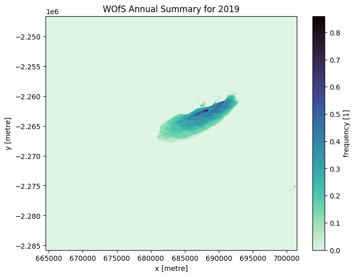
The plot below will have values that range from 0 to 1. Values that approach 1 indicate a permanent waterbody, while values closer to 0 indicate a more ephemeral or seasonal waterbody.
[10]:
wofs_annual.frequency.plot(size=6, cmap=sns.color_palette("mako_r", as_cmap=True))
plt.title('WOfS Annual Summary for 2019');
Loading WOfS ‘all-time’ summaries
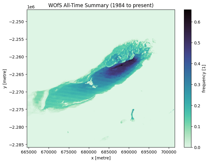
To look at a summary of WOFLs over the entire Landsat archive (around 1984 to present), we can load the wofs_ls_summary_alltime product.
[11]:
wofs_alltime = dc.load(product='wofs_ls_summary_alltime',
               like=wofls.geobox)

print(wofs_alltime)
<xarray.Dataset>
Dimensions:      (time: 1, y: 1306, x: 1231)
Coordinates:
  * time         (time) datetime64[ns] 2003-07-02T11:59:59.999999
  * y            (y) float64 -2.247e+06 -2.247e+06 ... -2.286e+06 -2.286e+06
  * x            (x) float64 6.646e+05 6.646e+05 ... 7.014e+05 7.015e+05
    spatial_ref  int32 32634
Data variables:
    count_wet    (time, y, x) int16 0 0 0 0 0 0 0 0 0 0 ... 0 0 0 0 0 0 0 0 0 0
    count_clear  (time, y, x) int16 557 558 558 558 559 ... 966 969 969 966 965
    frequency    (time, y, x) float32 0.0 0.0 0.0 0.0 0.0 ... 0.0 0.0 0.0 0.0
Attributes:
    crs:           PROJCS["WGS 84 / UTM zone 34N",GEOGCS["WGS 84",DATUM["WGS_...
    grid_mapping:  spatial_ref
Plot the WOfS all-time summary
[12]:
wofs_alltime.frequency.plot(size=6, cmap=sns.color_palette("mako_r", as_cmap=True))
plt.title('WOfS All-Time Summary (1984 to present)');
Additional information
License: The code in this notebook is licensed under the Apache License, Version 2.0. Digital Earth Africa data is licensed under the Creative Commons by Attribution 4.0 license.
Contact: If you need assistance, please post a question on the Open Data Cube Slack channel or on the GIS Stack Exchange using the open-data-cube tag (you can view previously asked questions here). If you would like to repoart an issue with this notebook, you can file one on
Github.
Compatible datacube version:
[13]:
print(datacube.__version__)
1.8.15
Last Tested:
[14]:
from datetime import datetime
datetime.today().strftime('%Y-%m-%d')
[14]:
'2023-08-11'