ALOS/ALOS-2 PALSAR/PALSAR-2 Annual Mosaics 
Products used: alos_palsar_mosaic, jers_sar_mosaic
Keywords data used; ALOS PALSAR, data used; ALOS-2 PALSAR-2, datasets; ALOS/ALOS-2 PALSAR/PALSAR-2, data used; JERS SAR, datasets; JERS SAR, index:SAR
Background
The ALOS/ALOS2 PALSAR Annual Mosaic is a global 25 m resolution dataset that combines data from many images captured by JAXA’s PALSAR and PALSAR-2 sensors on ALOS-1 and ALOS-2 satellites respectively. This product contains radar measurement in L-band and in HH and HV polarizations. It has a spatial resolution of 25m and is available annually for 2007 to 2010 (ALOS/PALSAR) and 2015 to 2022 (ALOS-2/PALSAR-2). ALOS/ALOS2 PALSAR mosaic data is part of a global dataset provided by the Japan Aerospace Exploration Agency (JAXA) Earth Observation Research Center. Historically, the JERS annual mosaic is generated from images acquired by the SAR sensor on the Japanese Earth Resources Satellite-1 (JERS-1) satellite.
DE Africa’s ALOS/ALOS-2 PALSAR/PALSAR-2 and JERS annual mosaic are Normalized Radar Backscatter data, for which Radiometric Terrain Correction (RTC) has been applied to data acquired with different imaging geometries over the same region.The relevant coverage and metadata of ALOS/ALOS2 PALSAR dataset can be viewed on DE Africa Metadata Explorer while JERS dataset coverage can be access via this link that forms a single, cohesive Analysis Ready Data (ARD) package, which allows you to analyse radar backscatter data as-is without the need to apply additional corrections.
Important details:
ALOS/ALOS2 PALSAR annual mosaic product specifications
Number of bands:
5To achieve backscatter in decibel unit, convert backscatter values in Digital Number (DN) using $ 10 * log10(DN^2) - 83.0 $
Mask specification includes
0forno-data,50for water,100for lay_over,150for shadowing and255for landObservation date is expressed as days after launch, which are Jan. 24, 2006 and May. 24, 2014 for PALSAR and PALSAR-2 respectively.
Native pixel alignment is
centreDate-range: selected years from 2007 to 2022
Spatial resolution: 25 x 25 m
JERS annual mosaic product specifications
Number of bands:
4To achieve backscatter in decibel unit, convert backscatter values in Digital Number (DN) using $ 10 * log10(DN^2) - 84.66 $
Mask specification includes
0forno-data,50for water,100for lay_over,150for shadowing and255for landObservation date is expressed as days after launch, which is Feb. 11, 1992 for JERS-1.
Native pixel alignment is
centreDate-range: 1996
Spatial resolution: 25 x 25 m
For a detailed description of DE Africa’s ALOS/ALOS2 PALSAR archive, see the DE Africa’s ALOS/ALOS2 technical specifications documentation.
Description
In this notebook we will load ALOS PALSAR data using dc.load() to return a time series of satellite images from a single sensor.
Topics covered include:
Inspecting the ALOS PALSAR products and measurements available in the datacube
Using the native
dc.load()function to load in dual polarization ALOS PALSAR data and visualizeUsing
dc.load()function to load single polarization JERS mosaic and visualize
Getting started
To run this analysis, run all the cells in the notebook, starting with the “Load packages” cell.
Load packages
[1]:
%matplotlib inline
import datacube
import sys
import math
import pandas as pd
import numpy as np
import xarray as xr
import matplotlib.pyplot as plt

from deafrica_tools.plotting import rgb
from deafrica_tools.datahandling import load_ard
from deafrica_tools.plotting import display_map
Connect to the datacube
[2]:
dc = datacube.Datacube(app="ALOS")
Available products and measurements
List products
We can use datacube’s list_products functionality to inspect DE Africa’s SAR products that are available in the datacube. The table below shows the product names that we will use to load the data, a brief description of the data, and the satellite instrument that acquired the data.
[3]:
dc.list_products().loc[dc.list_products()['description'].str.contains('SAR')]
[3]:
| name | description | license | default_crs | default_resolution | |
|---|---|---|---|---|---|
| name | |||||
| alos_palsar_mosaic | alos_palsar_mosaic | ALOS/PALSAR and ALOS-2/PALSAR-2 annual mosaic ... | None | EPSG:4326 | (-0.000222222222222, 0.000222222222222) |
| jers_sar_mosaic | jers_sar_mosaic | JERS-1 SAR annual mosaic tiles generated for u... | None | EPSG:4326 | (-0.000222222222222, 0.000222222222222) |
List measurements
We can further inspect the data available for each SAR product using datacube’s list_measurements functionality. The table below lists each of the measurements available in the data.
[4]:
productA = "alos_palsar_mosaic"
[5]:
measurements = dc.list_measurements()
measurements.loc[productA]
[5]:
| name | dtype | units | nodata | aliases | flags_definition | scale_factor | |
|---|---|---|---|---|---|---|---|
| measurement | |||||||
| hh | hh | uint16 | 1 | 0.0 | [hh] | NaN | NaN |
| hv | hv | uint16 | 1 | 0.0 | [hv] | NaN | NaN |
| date | date | uint16 | 1 | 0.0 | [date] | NaN | NaN |
| linci | linci | uint8 | 1 | 0.0 | [local incidence angle, linci, incidence] | NaN | NaN |
| mask | mask | uint8 | 1 | 0.0 | [mask] | {'category': {'bits': [0, 1, 2, 3, 4, 5, 6, 7]... | NaN |
Load ALOS PALSAR Annual Mosaic dataset using dc.load()
Now that we know what products and measurements are available for the products, we can load data from the datacube using dc.load.
In the example below, we will load ALOS PALSAR for Cairo and its surrounding in Egypt between 2007 and 2022.
We will load data from two polarizations, as well as the data mask ('mask') and observation date. The data is loaded in native EPSG:4326 coordinate reference system (CRS). It can be reprojected if output_crs and resolution are defined in the query.
Note: For a more general discussion of how to load data using the datacube, refer to the Introduction to loading data notebook.
[6]:
# Setting the query for area in the proximity of Cairo
lon = (31.90, 32.10)
lat = (30.37, 30.55)
query = {"x": lon,
         "y": lat,
         "time": ("2007", "2022")}
Visualise the selected area
[7]:
display_map(x=lon, y=lat)
[7]:
[8]:
#loading the data with the mask band included
bands = ['hh','hv','mask', 'date']
ds_ALOS = dc.load(product='alos_palsar_mosaic',
             measurements=bands,
             **query)

print(ds_ALOS)
<xarray.Dataset> Size: 61MB
Dimensions:      (time: 12, latitude: 811, longitude: 900)
Coordinates:
  * time         (time) datetime64[ns] 96B 2007-07-02T11:59:59.500000 ... 202...
  * latitude     (latitude) float64 6kB 30.55 30.55 30.55 ... 30.37 30.37 30.37
  * longitude    (longitude) float64 7kB 31.9 31.9 31.9 31.9 ... 32.1 32.1 32.1
    spatial_ref  int32 4B 4326
Data variables:
    hh           (time, latitude, longitude) uint16 18MB 2126 2712 ... 885 748
    hv           (time, latitude, longitude) uint16 18MB 802 915 ... 312 435
    mask         (time, latitude, longitude) uint8 9MB 255 255 255 ... 255 255
    date         (time, latitude, longitude) uint16 18MB 582 582 ... 2775 2775
Attributes:
    crs:           EPSG:4326
    grid_mapping:  spatial_ref
[9]:
#creation of a new band (HV/HH = hvhh) for RGB display
ds_ALOS['hvhh'] = ds_ALOS.hv / ds_ALOS.hh
[10]:
# Set the timesteps to visualise
timesteps = [0,5,10]

# Generate RGB plots at each timestep
rgb(ds_ALOS, bands=['hh','hv','hvhh'], index=timesteps)
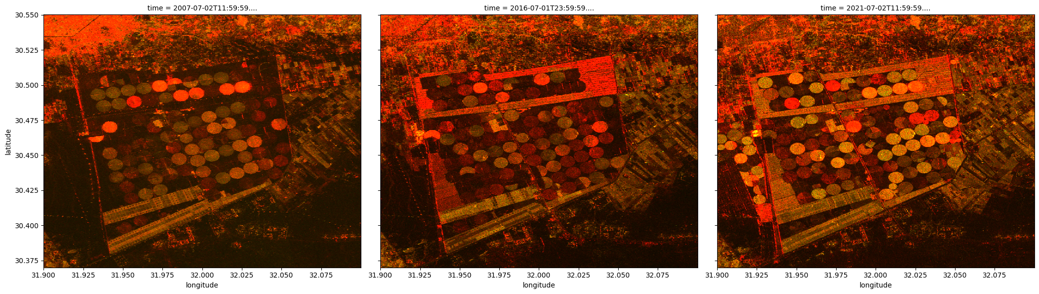
Inspection of observation date
Each annual mosaic is created from multiple oberservations from a year. This may result in discontinuity across images as seen above. It also means mosaics from different years may come from different seasons.
[11]:
# plot date for a mosaic
ds_ALOS.isel(time=3).date.plot.imshow(robust=True);
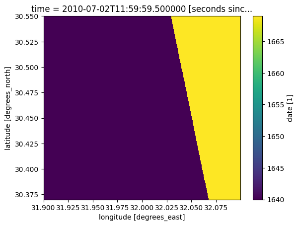
The observation date should be considered when evaluating change detected from year to year. In this example, we find the earliest, latest and median observation dates for each mosaic loaded.
[12]:
min_days = ds_ALOS.date.min(dim=['latitude','longitude']).values
max_days = ds_ALOS.date.max(dim=['latitude','longitude']).values
med_days = ds_ALOS.date.median(dim=['latitude','longitude']).astype(min_days.dtype).values
[13]:
# Define ALOS and ALOS-2 launch dates

alos_launch = np.datetime64('2006-01-24')
alos2_launch = np.datetime64('2014-05-24')
[14]:
# Calculate earliest, latest and median observation dates, using launch dates and offsets reported in the date band

indexed_time = ds_ALOS.time.values
min_dates = np.empty(len(indexed_time),dtype='<M8[D]')
max_dates = np.empty(len(indexed_time),dtype='<M8[D]')
med_dates = np.empty(len(indexed_time),dtype='<M8[D]')

for i, time in enumerate(indexed_time):
    if time < np.datetime64('2015'):
        min_dates[i] = alos_launch + np.timedelta64(min_days[i], 'D')
        max_dates[i] = alos_launch + np.timedelta64(max_days[i], 'D')
        med_dates[i] = alos_launch + np.timedelta64(med_days[i], 'D')
    else:
        min_dates[i] = alos2_launch + np.timedelta64(min_days[i], 'D')
        max_dates[i] = alos2_launch + np.timedelta64(max_days[i], 'D')
        med_dates[i] = alos2_launch + np.timedelta64(med_days[i], 'D')
The date ranges below show that the observations can span a few months. Occasionally data used may be from another year.
[15]:
for i in zip(min_dates, max_dates, (max_dates - min_dates).astype(int)): print("Date range and span (in days)", i)
Date range and span (in days) (numpy.datetime64('2007-06-27'), numpy.datetime64('2007-08-29'), 63)
Date range and span (in days) (numpy.datetime64('2008-08-31'), numpy.datetime64('2008-09-29'), 29)
Date range and span (in days) (numpy.datetime64('2009-08-17'), numpy.datetime64('2009-09-03'), 17)
Date range and span (in days) (numpy.datetime64('2010-07-22'), numpy.datetime64('2010-08-20'), 29)
Date range and span (in days) (numpy.datetime64('2015-07-07'), numpy.datetime64('2015-07-07'), 0)
Date range and span (in days) (numpy.datetime64('2016-07-05'), numpy.datetime64('2016-07-05'), 0)
Date range and span (in days) (numpy.datetime64('2017-07-04'), numpy.datetime64('2017-07-04'), 0)
Date range and span (in days) (numpy.datetime64('2018-03-27'), numpy.datetime64('2018-03-27'), 0)
Date range and span (in days) (numpy.datetime64('2019-01-01'), numpy.datetime64('2019-01-01'), 0)
Date range and span (in days) (numpy.datetime64('2020-12-29'), numpy.datetime64('2020-12-29'), 0)
Date range and span (in days) (numpy.datetime64('2021-12-28'), numpy.datetime64('2021-12-28'), 0)
Date range and span (in days) (numpy.datetime64('2021-12-28'), numpy.datetime64('2021-12-28'), 0)
[16]:
# Assign median dates to be the timestamps
ds_ALOS['time'] =  med_dates.astype('datetime64[ns]')
Coverting DN Values to Decibel Units
Since Backscatter data is provided as digital number(DN), it can be converted to backscatter in decibel unit to enhance contrast using the provided conversion equation. Before converting to decibel, we also apply the data mask to exclude pixels in radar shadow or with layerover.
[17]:
#convert DN to db values
ds_ALOS['hh_db'] =  10 * np.log10(ds_ALOS.hh.where(ds_ALOS.mask.isin([50,255]))**2) - 83.0
ds_ALOS['hv_db'] =  10 * np.log10(ds_ALOS.hv.where(ds_ALOS.mask.isin([50,255]))**2) - 83.0
ds_ALOS['hvhh_db'] = ds_ALOS['hv_db'] - ds_ALOS ['hh_db']
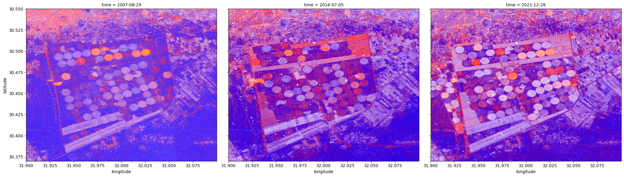
[18]:
# Set the timesteps to visualise
timesteps = [0,5,10]

# Generate RGB plots at each timestep
rgb(ds_ALOS, bands=['hh_db','hv_db','hvhh_db'], index=timesteps)
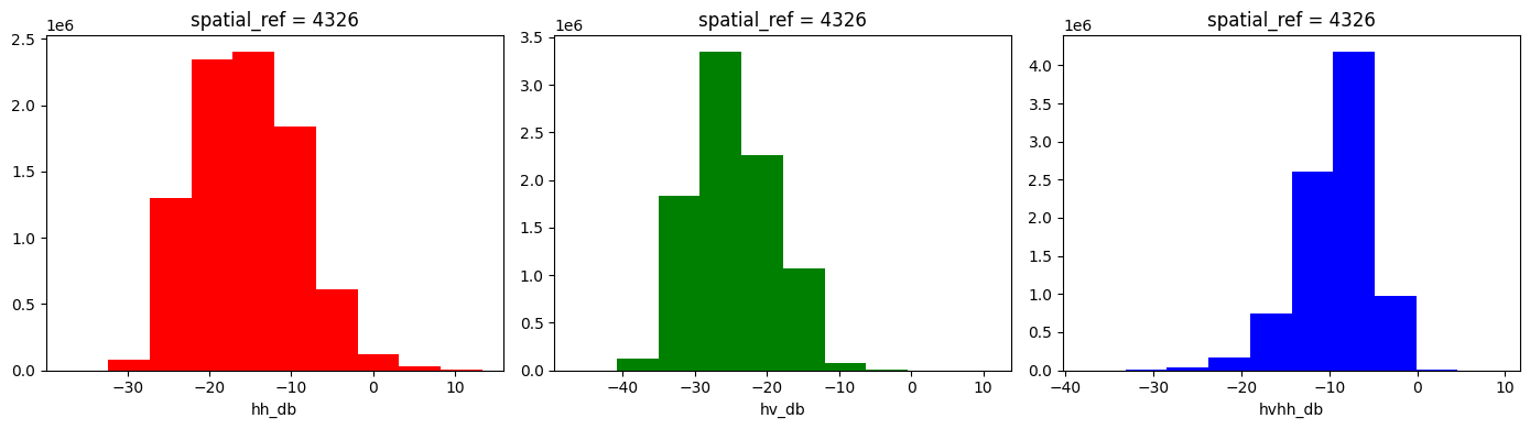
Histogram Analysis for ALOS/ALOS-2 PALSAR Dataset
Use histograms to inspect the distribution of backscatter values.
[19]:
#plotting each polorisation bands following converting to dB values
fig, ax = plt.subplots(1, 3, figsize=(14, 4))
ds_ALOS.hh_db.plot.hist(ax=ax[0], facecolor='red')
ds_ALOS.hv_db.plot.hist(ax=ax[1], facecolor='green')
ds_ALOS.hvhh_db.plot.hist(ax=ax[2], facecolor='blue')
plt.tight_layout()
Load JERS dataset using dc.load()
In the example below, we will load JERS annual mosaic for Cairo and its surrounding in Egypt in 1996.
We will load data from HH polarization, as well as the data mask (mask). The data is loaded in native EPSG:4326 coordinate reference system (CRS). It can be reprojected if output_crs and resolution are defined in the query.
Note: For a more general discussion of how to load data using the datacube, refer to the Introduction to loading data notebook.
[20]:
# Setting the query for area in the proximity of Cairo
lon = (31.90, 32.10)
lat = (30.37, 30.55)
query_jers = {"x": lon,
         "y": lat,
         "time": ("1996")}
[21]:
#loading the data with the mask band included
bands = ['hh','mask']
ds_JERS = dc.load(product='jers_sar_mosaic',
             measurements=bands,
             **query_jers)

print(ds_JERS)
<xarray.Dataset> Size: 2MB
Dimensions:      (time: 1, latitude: 811, longitude: 900)
Coordinates:
  * time         (time) datetime64[ns] 8B 1996-07-01T23:59:59.500000
  * latitude     (latitude) float64 6kB 30.55 30.55 30.55 ... 30.37 30.37 30.37
  * longitude    (longitude) float64 7kB 31.9 31.9 31.9 31.9 ... 32.1 32.1 32.1
    spatial_ref  int32 4B 4326
Data variables:
    hh           (time, latitude, longitude) uint16 1MB 6505 6953 ... 2750 2750
    mask         (time, latitude, longitude) uint8 730kB 255 255 255 ... 255 255
Attributes:
    crs:           EPSG:4326
    grid_mapping:  spatial_ref
[22]:
#convert DN values in JERS dataset to db values
ds_JERS['hh_db'] =  10 * np.log10(ds_JERS.hh.where(ds_JERS.mask.isin([50,255]))**2) - 84.66
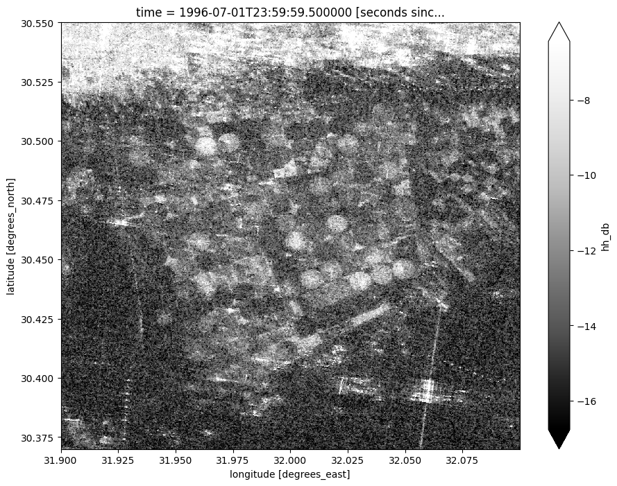
[23]:
# Plot all VH observations for the year
ds_JERS.hh_db.plot(cmap="Greys_r", robust=True,size=8);
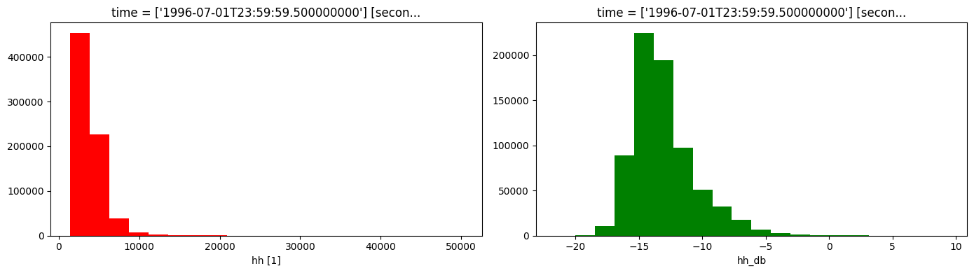
Histogram Analysis for JERS HH Polarization
Inspect backscatter distribution in this area
[24]:
#plotting each polorisation bands following converting to dB values
fig, ax = plt.subplots(1, 2, figsize=(14, 4))
ds_JERS.hh.plot.hist(ax=ax[0], bins=20, facecolor='red')
ds_JERS.hh_db.plot.hist(ax=ax[1], bins=20, facecolor='green')
plt.tight_layout()
Additional information
License: The code in this notebook is licensed under the Apache License, Version 2.0. Digital Earth Africa data is licensed under the Creative Commons by Attribution 4.0 license.
Contact: If you need assistance, please post a question on the Open Data Cube Slack channel or on the GIS Stack Exchange using the open-data-cube tag (you can view previously asked questions here). If you would like to report an issue with this notebook, you can file one on
Github.
Compatible datacube version:
[25]:
print(datacube.__version__)
1.8.20
Last Tested:
[26]:
from datetime import datetime
datetime.today().strftime('%Y-%m-%d')
[26]:
'2025-01-15'