Vegetation phenology in the Ruko Conservancy
Products used: s2_l2a
Background
Phenology is the study of plant and animal life cycles in the context of the seasons. It can be useful in understanding the life cycle trends of crops and how the growing seasons are affected by changes in climate. For more information, see the USGS page on deriving phenology.
Description
This notebook will produce annual, smoothed, one-dimensional (zonal mean across a region) time-series of a remote sensing vegetation indice, such as NDVI or EVI. In addition, basic phenology statistics are calculated, exported to disk as csv files, and annotated on a plot.
A number of steps are required to produce the desired outputs:
Load satellite data for a region specified by an vector file (shapefile or geojson)
Buffer the cloud masking layer to better mask clouds in the data (Sentinel-2 cloud mask is quite poor)
Further prepare the data for analysis by removing bad values (infs), masking surafce water, and removing outliers in the vegetation index.
Calculate a zonal mean across the study region (collapse the x and y dimension by taking the mean across all pixels for each time-step).
Interpolate and smooth the time-series to ensure a consistent dataset with all gaps and noise removed.
Calculate phenology statistics, report the results, save the results to disk, and generate an annotated plot.
Getting started
To run this analysis, run all the cells in the notebook, starting with the “Load packages” cell.
Load packages
Load key Python packages and supporting functions for the analysis.
[1]:
%matplotlib inline

import datetime as dt

import datacube
import geopandas as gpd
import matplotlib as mpl
import matplotlib.pyplot as plt
import mpl_toolkits.axisartist as AA
import numpy as np
import pandas as pd
import xarray as xr
from odc.geo.geom import Geometry
from datacube.utils.aws import configure_s3_access
from mpl_toolkits.axes_grid1 import host_subplot

from deafrica_tools.bandindices import calculate_indices
from deafrica_tools.classification import HiddenPrints
from deafrica_tools.dask import create_local_dask_cluster
from deafrica_tools.datahandling import load_ard
from deafrica_tools.plotting import map_shapefile
from deafrica_tools.spatial import xr_rasterize
import deafrica_tools.temporal as ts

configure_s3_access(aws_unsigned=True, cloud_defaults=True)
Set up a Dask cluster
Dask can be used to better manage memory use and conduct the analysis in parallel. For an introduction to using Dask with Digital Earth Africa, see the Dask notebook.
Note: We recommend opening the Dask processing window to view the different computations that are being executed; to do this, see the Dask dashboard in DE Africa section of the Dask notebook.
To use Dask, set up the local computing cluster using the cell below.
[2]:
create_local_dask_cluster(spare_mem='2Gb')
Client
Client-be3a70f2-43c5-11f1-9d4d-ae180e9931c9
| Connection method: Cluster object | Cluster type: distributed.LocalCluster |
| Dashboard: /user/mpho.sadiki@digitalearthafrica.org/proxy/8787/status |
Cluster Info
LocalCluster
a6f87acb
| Dashboard: /user/mpho.sadiki@digitalearthafrica.org/proxy/8787/status | Workers: 1 |
| Total threads: 4 | Total memory: 27.14 GiB |
| Status: running | Using processes: True |
Scheduler Info
Scheduler
Scheduler-c5b2d8b2-65f1-4adb-b2f7-d6edbce2b80d
| Comm: tcp://127.0.0.1:37547 | Workers: 0 |
| Dashboard: /user/mpho.sadiki@digitalearthafrica.org/proxy/8787/status | Total threads: 0 |
| Started: Just now | Total memory: 0 B |
Workers
Worker: 0
| Comm: tcp://127.0.0.1:33581 | Total threads: 4 |
| Dashboard: /user/mpho.sadiki@digitalearthafrica.org/proxy/46879/status | Memory: 27.14 GiB |
| Nanny: tcp://127.0.0.1:34867 | |
| Local directory: /tmp/dask-scratch-space/worker-p4co7pwb | |
Analysis parameters
The following cell sets important parameters for the analysis:
veg_proxy: Band index to use as a proxy for vegetation health e.g.'NDVI'or'EVI'product: The satellite product to load. Either Sentinel-2:'s2_l2a', or Landsat-8:'ls8_cl2'shapefile: The path to the vector file delineating the analysis region. Can be a shapefile or a geojsontime_range: The year range to analyse (e.g.('2017-01-01', '2019-12-30')).min_gooddata: the fraction of good data (not cloudy) a scene must have before it is returned as a datasetresolution: The pixel resolution, in metres, of the returned datasetdask_chunks: The size, in number of pixel, for the dask chunks on each dimension.
[3]:
veg_proxy = 'NDVI'

product = 's2_l2a'

shapefile='data/Ruko_conservancy.geojson'

time_range = ('2017-01-01', '2020-12-31')

resolution = (-20,20)

dask_chunks = {'x':500, 'y':500}
Connect to the datacube
Connect to the datacube so we can access DE Africa data. The app parameter is a unique name for the analysis which is based on the notebook file name.
[4]:
dc = datacube.Datacube(app='Vegetation_phenology')
View the region of interest
The next cell will display the selected area on an web map.
[5]:
#First open the shapefile using geopandas
gdf = gpd.read_file(shapefile)
[6]:
map_shapefile(gdf, attribute='ConsrvName')
Load cloud-masked Sentinel-2 data
The first step is to load Sentinel-2 data for the specified area of interest and time range. The load_ard function is used here to load data that has been masked for cloud, shadow and quality filters, making it ready for analysis.
The cell directly below will create a query object using the first geometry in the shapefile, along with the parameters we defined in the Analysis Parameters section above.
[7]:
# Create a reusable query
geom = Geometry(geom=gdf.iloc[0].geometry, crs=gdf.crs)

query = {
    "geopolygon": geom,
    'time': time_range,
    'measurements': ['red','nir','green','swir_1'],
    'resolution': resolution,
    'output_crs': 'epsg:6933',
    'group_by':'solar_day'
}
Load available data from S2. The cloud masking data for Sentinel-2 is less than perfect, and missed cloud in the data greatly impacts vegetation calculations. load_ard supports morphological operations on the cloud-masking bands to improve the masking of poor quality data.
[8]:
filters=[("opening", 3), ("dilation", 2)]

ds = load_ard(
    dc=dc,
    products=['s2_l2a'],
    dask_chunks=dask_chunks,
    mask_filters=filters,
    **query,
)

print(ds)
Using pixel quality parameters for Sentinel 2
Finding datasets
    s2_l2a
Applying morphological filters to pq mask [('opening', 3), ('dilation', 2)]
Applying pixel quality/cloud mask
Returning 267 time steps as a dask array
<xarray.Dataset> Size: 3GB
Dimensions:      (time: 267, y: 1194, x: 607)
Coordinates:
  * time         (time) datetime64[ns] 2kB 2017-01-02T08:07:11 ... 2020-12-27...
  * y            (y) float64 10kB 9.461e+04 9.459e+04 ... 7.077e+04 7.075e+04
  * x            (x) float64 5kB 3.479e+06 3.479e+06 ... 3.491e+06 3.491e+06
    spatial_ref  int32 4B 6933
Data variables:
    red          (time, y, x) float32 774MB dask.array<chunksize=(1, 500, 500), meta=np.ndarray>
    nir          (time, y, x) float32 774MB dask.array<chunksize=(1, 500, 500), meta=np.ndarray>
    green        (time, y, x) float32 774MB dask.array<chunksize=(1, 500, 500), meta=np.ndarray>
    swir_1       (time, y, x) float32 774MB dask.array<chunksize=(1, 500, 500), meta=np.ndarray>
Attributes:
    crs:           EPSG:6933
    grid_mapping:  spatial_ref
/opt/venv/lib/python3.12/site-packages/odc/algo/_masking.py:425: FutureWarning: `binary_opening` is deprecated since version 0.26 and will be removed in version 0.28. Use `skimage.morphology.opening` instead.
  mask = op(mask, _disk(radius, mask.ndim))
/opt/venv/lib/python3.12/site-packages/odc/algo/_masking.py:425: FutureWarning: `binary_dilation` is deprecated since version 0.26 and will be removed in version 0.28. Use `skimage.morphology.dilation` instead. Note the lack of mirroring for non-symmetric footprints (see docstring notes).
  mask = op(mask, _disk(radius, mask.ndim))
/opt/venv/lib/python3.12/site-packages/deafrica_tools/datahandling.py:565: FutureWarning: In a future version of xarray the default value for compat will change from compat='no_conflicts' to compat='override'. This is likely to lead to different results when combining overlapping variables with the same name. To opt in to new defaults and get rid of these warnings now use `set_options(use_new_combine_kwarg_defaults=True) or set compat explicitly.
  ds = xr.merge([ds_data, ds_masks])
Mask the satellite data with shape
[9]:
#create mask
mask = xr_rasterize(gdf,ds)

#mask data
ds = ds.where(mask)

#convert to float 32 to conserve memory
ds=ds.astype(np.float32)
Calculate vegetation and water indices
[10]:
# Calculate the chosen vegetation proxy index and add it to the loaded data set
ds = calculate_indices(ds, index=[veg_proxy, 'MNDWI'], satellite_mission='s2', drop=True)
Dropping bands ['red', 'nir', 'green', 'swir_1']
Prepare data for analysis
Remove any NaN or infinite values, mask water, remove any outliers in the vegetation index. We then reduce the data to a 1D timeseries by calculating the mean across the x and y dimensions.
We will also ‘compute’ the data on the dask cluster to speed up calculations later on. This step will take 5-10mins to run since we are now computing everything that came before.
[11]:
# remove any infinite values
ds = ds.where(~np.isinf(ds))
# mask water
ds = ds.where(ds.MNDWI < 0)

#remove outliers (if NDVI greater than 1.0, set to NaN, if less than 0 set to NaN)
ds[veg_proxy] = xr.where(ds[veg_proxy]>1.0, np.nan, ds[veg_proxy])
ds[veg_proxy] = xr.where(ds[veg_proxy]<0, np.nan, ds[veg_proxy])

# create 1D line plots
veg = ds[veg_proxy].mean(['x', 'y']).compute()
/opt/venv/lib/python3.12/site-packages/odc/algo/_masking.py:425: FutureWarning: `binary_opening` is deprecated since version 0.26 and will be removed in version 0.28. Use `skimage.morphology.opening` instead.
  mask = op(mask, _disk(radius, mask.ndim))
/opt/venv/lib/python3.12/site-packages/odc/algo/_masking.py:425: FutureWarning: `binary_dilation` is deprecated since version 0.26 and will be removed in version 0.28. Use `skimage.morphology.dilation` instead. Note the lack of mirroring for non-symmetric footprints (see docstring notes).
  mask = op(mask, _disk(radius, mask.ndim))
/opt/venv/lib/python3.12/site-packages/rasterio/warp.py:385: NotGeoreferencedWarning: Dataset has no geotransform, gcps, or rpcs. The identity matrix will be returned.
  dest = _reproject(
Smooth and interpolate time series
Due to many factors (e.g. cloud obscuring the region, missed cloud cover in the SCL layer) the data will be gappy and noisy. Here, we will smooth and interpolate the data to ensure we working with a consistent time-series.
To do this we take two steps:
Resample the data to fortnightly time-steps using the fortnightly median
Calculate a rolling mean with a window of 4 steps
[12]:
resample_period='2W'
window=4

veg_smooth = veg.resample(time=resample_period, label='left').median().rolling(time=window, min_periods=1).mean()
# Update the time coordinates of the resampled dataset.
veg_smooth = veg_smooth.assign_coords(time=(veg_smooth.time + np.timedelta64(1, 'W')))
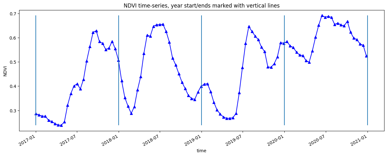
Plot the entire time-series
[13]:
veg_smooth.plot.line('b-^', figsize=(15,5))
_max=veg_smooth.max()
_min=veg_smooth.min()
plt.vlines(np.datetime64('2017-01-01'), ymin=_min, ymax=_max)
plt.vlines(np.datetime64('2018-01-01'), ymin=_min, ymax=_max)
plt.vlines(np.datetime64('2019-01-01'), ymin=_min, ymax=_max)
plt.vlines(np.datetime64('2020-01-01'), ymin=_min, ymax=_max)
plt.vlines(np.datetime64('2021-01-01'), ymin=_min, ymax=_max)
plt.title(veg_proxy+' time-series, year start/ends marked with vertical lines')
plt.ylabel(veg_proxy);
Compute basic phenology statistics
Below we specify the statistics to calculate, and the method we’ll use for determining the statistics.
The statistics acronyms are as follows:
SOS- Date of Start of SeasonvSOS- value at Start of SeasonPOS- Date of Peak of SeasonvPOS- value at Peak of SeasonEOS- Date of End of SeasonvEOS- value at End of SeasonTrough- minimum value across the dataset timeframeLOS- Length of Season, measured in daysAOS- Amplitude of Season, the difference betweenvPOSandTroughROG- Rate of Greening, rate of change from start to peak of seasonROS- Rate of Senescing, rae of change from peak to end of season
Options are ‘first’ & ‘median’ for method_sos, and ‘last’ & ‘median’ for method_eos.
method_sos : str
        If 'first' then vSOS is estimated as the first positive
        slope on the greening side of the curve. If 'median',
        then vSOS is estimated as the median value of the postive
        slopes on the greening side of the curve.

method_eos : str
        If 'last' then vEOS is estimated as the last negative slope
        on the senescing side of the curve. If 'median', then vEOS is
        estimated as the 'median' value of the negative slopes on the
        senescing side of the curve.
[14]:
basic_pheno_stats = ['SOS','vSOS','POS','vPOS','EOS','vEOS','Trough','LOS','AOS','ROG','ROS']
method_sos = 'first'
method_eos = 'last'
[15]:
# find all the years to assist with plotting
years=veg_smooth.groupby("time.year")

# get list of years in ts to help with looping
years_int = [y[0] for y in years]

# store results in dict
pheno_results = {}

# loop through years and calculate phenology
for year in years_int:
    # select year
    da = dict(years)[year]

    # calculate stats
    stats = ts.xr_phenology(
        da,
        method_sos=method_sos,
        method_eos=method_eos,
        stats=basic_pheno_stats,
        verbose=False,
    )
    # add results to dict
    pheno_results[str(year)] = stats
Print the phenology statistics for each year, and write the results to disk as a .csv
[16]:
df_dict = {}
for key, value in pheno_results.items():
    df_dict_1 = {}
    for b in value.data_vars:
        if value[b].dtype == np.dtype("<M8[ns]") or value[b].dtype == np.dtype("int16"):
            result = pd.to_datetime(value[b].values)
        else:
            result = round(float(value[b].values), 3)
        df_dict_1[b] = result
    df_dict[key] = df_dict_1

df = (pd.DataFrame(df_dict)).T
df.to_csv('results/'+key+'_phenology.csv')
df
[16]:
| SOS | vSOS | POS | vPOS | EOS | vEOS | Trough | LOS | AOS | ROG | ROS | |
|---|---|---|---|---|---|---|---|---|---|---|---|
| 2017 | 2017-04-23 00:00:00 | 0.238 | 2017-09-24 00:00:00 | 0.629 | 2017-12-31 00:00:00 | 0.507 | 0.238 | 252.0 | 0.39 | 0.003 | -0.001 |
| 2018 | 2018-03-11 00:00:00 | 0.315 | 2018-07-15 00:00:00 | 0.655 | 2018-11-18 00:00:00 | 0.349 | 0.287 | 252.0 | 0.368 | 0.003 | -0.002 |
| 2019 | 2019-05-05 00:00:00 | 0.274 | 2019-07-28 00:00:00 | 0.656 | 2019-11-03 00:00:00 | 0.482 | 0.271 | 182.0 | 0.385 | 0.005 | -0.002 |
| 2020 | 2020-04-19 00:00:00 | 0.499 | 2020-07-26 00:00:00 | 0.696 | 2020-12-27 00:00:00 | 0.53 | 0.499 | 252.0 | 0.196 | 0.002 | -0.001 |
Annotate phenology on a plot
This image will be saved to disk in the results/ folder
[17]:
# Figure to which the subplot will be added
fig = plt.figure(figsize=(15, 7))
# Create a subplot that can act as a host to parasitic axes
host = host_subplot(111, figure=fig, axes_class=AA.Axes)
# fig, ax = plt.subplots()


# Function to use to edit the axes of the plot
def adjust_axes(ax):
    # Set the location of the major and minor ticks.
    ax.xaxis.set_major_locator(mpl.dates.MonthLocator())
    ax.xaxis.set_minor_locator(mpl.dates.MonthLocator(bymonthday=16))

    # Format the major and minor tick labels.

    ax.xaxis.set_major_formatter(mpl.ticker.NullFormatter())
    ax.xaxis.set_minor_formatter(mpl.dates.DateFormatter("%b"))


#     # Turn off unnecessary ticks.
    ax.axis["bottom"].minor_ticks.set_visible(False)

    ax.axis["top"].major_ticks.set_visible(False)
    ax.axis["top"].minor_ticks.set_visible(False)

    ax.axis["right"].major_ticks.set_visible(False)
    ax.axis["right"].minor_ticks.set_visible(False)


# find all the years to assist with plotting
years=veg_smooth.groupby('time.year')

# Counter to aid in plotting.
counter = 0

for y, year in years:
    # Grab all the values we need for plotting.
    eos = df.loc[str(y)].EOS
    sos = df.loc[str(y)].SOS
    pos = df.loc[str(y)].POS

    veos = df.loc[str(y)].vEOS
    vsos = df.loc[str(y)].vSOS
    vpos = df.loc[str(y)].vPOS

    if counter == 0:
        ax = host
    else:
        # Create the secondary axis.
        ax = host.twiny()

    # Plot the data
    year.plot(ax=ax, label=y)
    # add start of season

    ax.plot(sos, vsos, "or")
    ax.annotate(
        "SOS",
        xy=(sos, vsos),
        xytext=(-15, 20),
        textcoords="offset points",
        arrowprops=dict(arrowstyle="-|>"),
    )

    # add end of season
    ax.plot(eos, veos, "or")
    ax.annotate(
        "EOS",
        xy=(eos, veos),
        xytext=(0, 20),
        textcoords="offset points",
        arrowprops=dict(arrowstyle="-|>"),
    )

    # add peak of season
    ax.plot(pos, vpos, "or")
    ax.annotate(
        "POS",
        xy=(pos, vpos),
        xytext=(-10, -25),
        textcoords="offset points",
        arrowprops=dict(arrowstyle="-|>"),
    )

    # Set the x-axis limits
    min_x = dt.date(y, 1, 1)
    max_x = dt.date(y, 12, 31)
    ax.set_xlim(min_x, max_x)

    adjust_axes(ax)
    counter += 1


host.legend(labelcolor="linecolor")
host.set_ylim([_min - 0.025, _max.values + 0.05])

plt.ylabel(veg_proxy)
plt.xlabel("Month")

plt.title("Yearly " + veg_proxy);
plt.savefig('results/yearly_phenology_plot.png');
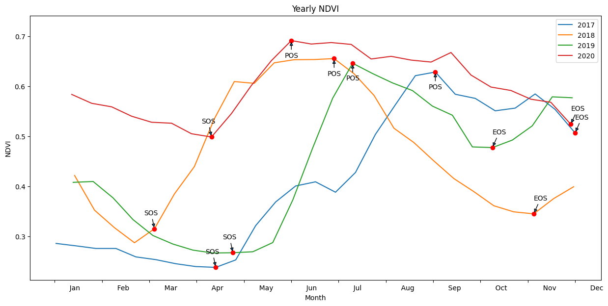
The basic phenology statistics are summarised in a more readable format below. We can compare the statistics at a high level. Further analysis should be conducted using the .csv exports in the /results folder.
[18]:
print(xr.concat([pheno_results[str(year)] for year in years_int],
                dim=pd.Index(years_int, name='time')).to_dataframe().drop(columns=['spatial_ref']).T.to_string())
time                   2017                 2018                 2019                 2020
SOS     2017-04-23 00:00:00  2018-03-11 00:00:00  2019-05-05 00:00:00  2020-04-19 00:00:00
vSOS               0.238188              0.31534             0.273537              0.49939
POS     2017-09-24 00:00:00  2018-07-15 00:00:00  2019-07-28 00:00:00  2020-07-26 00:00:00
vPOS               0.628646             0.655491             0.655767             0.695777
EOS     2017-12-31 00:00:00  2018-11-18 00:00:00  2019-11-03 00:00:00  2020-12-27 00:00:00
vEOS                0.50702             0.349192             0.481802             0.530077
Trough             0.238188             0.287414             0.271097              0.49939
LOS                   252.0                252.0                182.0                252.0
AOS                0.390459             0.368077              0.38467             0.196387
ROG                0.002535               0.0027              0.00455             0.002004
ROS               -0.001241            -0.002431            -0.001775            -0.001076
Additional information
License: The code in this notebook is licensed under the Apache License, Version 2.0. Digital Earth Africa data is licensed under the Creative Commons by Attribution 4.0 license.
Contact: If you need assistance, please post a question on the Open Data Cube Slack channel or on the GIS Stack Exchange using the open-data-cube tag (you can view previously asked questions here). If you would like to report an issue with this notebook, you can file one on
Github.
Compatible datacube version:
[19]:
print(datacube.__version__)
1.9.13
Last Tested:
[20]:
from datetime import datetime
datetime.today().strftime('%Y-%m-%d')
[20]:
'2026-04-29'