Parallel processing with Dask
Keywords
Background
Dask is a useful tool when working with large analyses (either in space or time) as it breaks data into manageable chunks that can be easily stored in memory. It can also use multiple computing cores to speed up computations. This has numerous benefits for analyses, which will be covered in this notebook.
Description
This notebook covers how to enable Dask as part of loading data, which can allow you to analyse larger areas and longer time-spans without crashing the DE Africa Environment, as well as potentially speeding up your calculations.
Topics covered in this notebook include:
The difference between the standard load command and loading with Dask.
Enabling Dask and the Dask Dashboard.
Setting chunk sizes for data loading.
Loading data with Dask.
Chaining operations together before loading any data and understanding task graphs.
Getting started
To run this introduction to Dask, run all the cells in the notebook starting with the “Load packages” cell. For help with running notebook cells, refer back to the Jupyter Notebooks notebook
Load packages
The cell below imports the datacube deafrica_tools dask create_local_dask_cluster
Connect to the datacube
The next step is to connect to the datacube database. The resulting dc app
Standard load
By default, the datacube not use Dask when loading data. This means that when dc.load()
For very large areas or long time spans, this can cause the Jupyter notebook to crash.
For more information on how to use dc.load() Loading data from DE Africa notebook
<xarray.Dataset>
Dimensions:      (time: 1, y: 17925, x: 14473)
Coordinates:
  * time         (time) datetime64[ns] 2018-07-02T11:59:59.999999
  * y            (y) float64 -2.501e+06 -2.501e+06 ... -2.681e+06 -2.681e+06
  * x            (x) float64 2.316e+06 2.316e+06 2.316e+06 ... 2.46e+06 2.46e+06
    spatial_ref  int32 6933
Data variables:
    red          (time, y, x) uint16 1083 1139 1208 1219 ... 1585 1687 1641 1596
    green        (time, y, x) uint16 900 934 992 1001 ... 1102 1176 1154 1131
    blue         (time, y, x) uint16 668 701 753 761 774 ... 686 727 766 759 726
Attributes:
    crs:           epsg:6933
grid_mapping: spatial_ref Dimensions:
Coordinates: (4)
time
(time)
datetime64[ns]
2018-07-02T11:59:59.999999
units : seconds since 1970-01-01 00:00:00 array(['2018-07-02T11:59:59.999999000'], dtype='datetime64[ns]') y
(y)
float64
-2.501e+06 ... -2.681e+06
units : metre resolution : -10.0 crs : epsg:6933 array([-2501275., -2501285., -2501295., ..., -2680495., -2680505., -2680515.]) x
(x)
float64
2.316e+06 2.316e+06 ... 2.46e+06
units : metre resolution : 10.0 crs : epsg:6933 array([2315675., 2315685., 2315695., ..., 2460375., 2460385., 2460395.]) spatial_ref
()
int32
6933
spatial_ref : PROJCS["WGS 84 / NSIDC EASE-Grid 2.0 Global",GEOGCS["WGS 84",DATUM["WGS_1984",SPHEROID["WGS 84",6378137,298.257223563,AUTHORITY["EPSG","7030"]],AUTHORITY["EPSG","6326"]],PRIMEM["Greenwich",0,AUTHORITY["EPSG","8901"]],UNIT["degree",0.0174532925199433,AUTHORITY["EPSG","9122"]],AUTHORITY["EPSG","4326"]],PROJECTION["Cylindrical_Equal_Area"],PARAMETER["standard_parallel_1",30],PARAMETER["central_meridian",0],PARAMETER["false_easting",0],PARAMETER["false_northing",0],UNIT["metre",1,AUTHORITY["EPSG","9001"]],AXIS["Easting",EAST],AXIS["Northing",NORTH],AUTHORITY["EPSG","6933"]] grid_mapping_name : lambert_cylindrical_equal_area Data variables: (3)
red
(time, y, x)
uint16
1083 1139 1208 ... 1687 1641 1596
units : 1 nodata : 0 crs : epsg:6933 grid_mapping : spatial_ref array([[[1083, 1139, 1208, ..., 962, 931, 942],
[1136, 1163, 1218, ..., 983, 980, 892],
[1213, 1176, 1205, ..., 963, 994, 948],
...,
[1701, 1724, 1734, ..., 1608, 1421, 1369],
[1696, 1719, 1729, ..., 1635, 1569, 1517],
[1687, 1701, 1718, ..., 1687, 1641, 1596]]], dtype=uint16) green
(time, y, x)
uint16
900 934 992 1001 ... 1176 1154 1131
units : 1 nodata : 0 crs : epsg:6933 grid_mapping : spatial_ref array([[[ 900, 934, 992, ..., 789, 765, 784],
[ 937, 945, 993, ..., 811, 806, 753],
[ 989, 951, 978, ..., 785, 815, 789],
...,
[1262, 1275, 1289, ..., 1123, 999, 960],
[1258, 1274, 1287, ..., 1132, 1093, 1071],
[1252, 1262, 1275, ..., 1176, 1154, 1131]]], dtype=uint16) blue
(time, y, x)
uint16
668 701 753 761 ... 727 766 759 726
units : 1 nodata : 0 crs : epsg:6933 grid_mapping : spatial_ref array([[[668, 701, 753, ..., 584, 562, 575],
[702, 706, 746, ..., 607, 603, 548],
[740, 703, 730, ..., 576, 606, 589],
...,
[893, 907, 914, ..., 720, 656, 632],
[887, 905, 913, ..., 733, 725, 692],
[883, 895, 905, ..., 766, 759, 726]]], dtype=uint16) Indexes: (3)
PandasIndex
PandasIndex(DatetimeIndex(['2018-07-02 11:59:59.999999'], dtype='datetime64[ns]', name='time', freq=None)) PandasIndex
PandasIndex(Index([-2501275.0, -2501285.0, -2501295.0, -2501305.0, -2501315.0, -2501325.0,
       -2501335.0, -2501345.0, -2501355.0, -2501365.0,
       ...
       -2680425.0, -2680435.0, -2680445.0, -2680455.0, -2680465.0, -2680475.0,
       -2680485.0, -2680495.0, -2680505.0, -2680515.0],
dtype='float64', name='y', length=17925)) PandasIndex
PandasIndex(Index([2315675.0, 2315685.0, 2315695.0, 2315705.0, 2315715.0, 2315725.0,
       2315735.0, 2315745.0, 2315755.0, 2315765.0,
       ...
       2460305.0, 2460315.0, 2460325.0, 2460335.0, 2460345.0, 2460355.0,
       2460365.0, 2460375.0, 2460385.0, 2460395.0],
      dtype='float64', name='x', length=14473))
Attributes: (2)
crs : epsg:6933 grid_mapping : spatial_ref
Enabling Dask
One of the major features of Dask is that it can take advantage of multiple CPU cores to speed up computations, which is known as distributed computing. This is good for situations where you need to do a lot of calculations on large datasets.
To set up distributed computing with Dask, you need to first set up a Dask client using the function below:
A print out should appear, displaying information about the Client Cluster Dashboard: heading, which should look something like /user/<email>/proxy/8787/status <email>
This link provides a way for you to view how any computations you run are progressing. There are two ways to view the dashboard:
Click the link, which will open a new tab in your browser
Set up the dashboard inside the DE Africa Environment.
We’ll now cover how to do the second option.
Dask dashboard in DE Africa
On the left-hand menu bar, click the Dask icon, as shown below:
Copy and paste the Dashboard link from the Client print out in the DASK DASHBOARD URL text box:
If the url is valid, the buttons should go from grey to orange. Click the orange PROGRESS button on the dask panel, which will open a new tab inside the DE Africa Environment.
To view the Dask window and your active notebook at the same time, drag the new Dask Progress tab to the bottom of the screen.
Now, when you do computations with Dask, you’ll see the progress of the computations in this new Dask window.
Lazy load
When using Dask, the dc.load()
Lazy-loading changes the data structure returned from the dc.load() xarray.Dataset dask.array
To request lazy-loaded data, add a dask_chunks dc.load()
<xarray.Dataset>
Dimensions:      (time: 1, y: 17925, x: 14473)
Coordinates:
  * time         (time) datetime64[ns] 2018-07-02T11:59:59.999999
  * y            (y) float64 -2.501e+06 -2.501e+06 ... -2.681e+06 -2.681e+06
  * x            (x) float64 2.316e+06 2.316e+06 2.316e+06 ... 2.46e+06 2.46e+06
    spatial_ref  int32 6933
Data variables:
    red          (time, y, x) uint16 dask.array<chunksize=(1, 3000, 3000), meta=np.ndarray>
    green        (time, y, x) uint16 dask.array<chunksize=(1, 3000, 3000), meta=np.ndarray>
    blue         (time, y, x) uint16 dask.array<chunksize=(1, 3000, 3000), meta=np.ndarray>
Attributes:
    crs:           epsg:6933
grid_mapping: spatial_ref Dimensions:
Coordinates: (4)
time
(time)
datetime64[ns]
2018-07-02T11:59:59.999999
units : seconds since 1970-01-01 00:00:00 array(['2018-07-02T11:59:59.999999000'], dtype='datetime64[ns]') y
(y)
float64
-2.501e+06 ... -2.681e+06
units : metre resolution : -10.0 crs : epsg:6933 array([-2501275., -2501285., -2501295., ..., -2680495., -2680505., -2680515.]) x
(x)
float64
2.316e+06 2.316e+06 ... 2.46e+06
units : metre resolution : 10.0 crs : epsg:6933 array([2315675., 2315685., 2315695., ..., 2460375., 2460385., 2460395.]) spatial_ref
()
int32
6933
spatial_ref : PROJCS["WGS 84 / NSIDC EASE-Grid 2.0 Global",GEOGCS["WGS 84",DATUM["WGS_1984",SPHEROID["WGS 84",6378137,298.257223563,AUTHORITY["EPSG","7030"]],AUTHORITY["EPSG","6326"]],PRIMEM["Greenwich",0,AUTHORITY["EPSG","8901"]],UNIT["degree",0.0174532925199433,AUTHORITY["EPSG","9122"]],AUTHORITY["EPSG","4326"]],PROJECTION["Cylindrical_Equal_Area"],PARAMETER["standard_parallel_1",30],PARAMETER["central_meridian",0],PARAMETER["false_easting",0],PARAMETER["false_northing",0],UNIT["metre",1,AUTHORITY["EPSG","9001"]],AXIS["Easting",EAST],AXIS["Northing",NORTH],AUTHORITY["EPSG","6933"]] grid_mapping_name : lambert_cylindrical_equal_area Data variables: (3)
red
(time, y, x)
uint16
dask.array<chunksize=(1, 3000, 3000), meta=np.ndarray>
units : 1 nodata : 0 crs : epsg:6933 grid_mapping : spatial_ref
Array
Chunk
Bytes
494.82 MiB
17.17 MiB
Shape
(1, 17925, 14473)
(1, 3000, 3000)
Dask graph
30 chunks in 1 graph layer
Data type
uint16 numpy.ndarray
14473
17925
1
green
(time, y, x)
uint16
dask.array<chunksize=(1, 3000, 3000), meta=np.ndarray>
units : 1 nodata : 0 crs : epsg:6933 grid_mapping : spatial_ref
Array
Chunk
Bytes
494.82 MiB
17.17 MiB
Shape
(1, 17925, 14473)
(1, 3000, 3000)
Dask graph
30 chunks in 1 graph layer
Data type
uint16 numpy.ndarray
14473
17925
1
blue
(time, y, x)
uint16
dask.array<chunksize=(1, 3000, 3000), meta=np.ndarray>
units : 1 nodata : 0 crs : epsg:6933 grid_mapping : spatial_ref
Array
Chunk
Bytes
494.82 MiB
17.17 MiB
Shape
(1, 17925, 14473)
(1, 3000, 3000)
Dask graph
30 chunks in 1 graph layer
Data type
uint16 numpy.ndarray
14473
17925
1
Indexes: (3)
PandasIndex
PandasIndex(DatetimeIndex(['2018-07-02 11:59:59.999999'], dtype='datetime64[ns]', name='time', freq=None)) PandasIndex
PandasIndex(Index([-2501275.0, -2501285.0, -2501295.0, -2501305.0, -2501315.0, -2501325.0,
       -2501335.0, -2501345.0, -2501355.0, -2501365.0,
       ...
       -2680425.0, -2680435.0, -2680445.0, -2680455.0, -2680465.0, -2680475.0,
       -2680485.0, -2680495.0, -2680505.0, -2680515.0],
dtype='float64', name='y', length=17925)) PandasIndex
PandasIndex(Index([2315675.0, 2315685.0, 2315695.0, 2315705.0, 2315715.0, 2315725.0,
       2315735.0, 2315745.0, 2315755.0, 2315765.0,
       ...
       2460305.0, 2460315.0, 2460325.0, 2460335.0, 2460345.0, 2460355.0,
       2460365.0, 2460375.0, 2460385.0, 2460395.0],
      dtype='float64', name='x', length=14473))
Attributes: (2)
crs : epsg:6933 grid_mapping : spatial_ref
The function should return much faster, as it is not reading any data from disk.
Dask chunks
After adding the dask_chunks dc.load() dask.array chunksize chunksize dask_chunks dc.load()
Dask works by breaking up large datasets into chunks, which can be read individually. You may specify the number of pixels in each chunk for each dataset dimension.
For example, we passed the following chunk definition to dc.load()
This definition tells Dask to cut the data into chunks containing 3000 pixels in the x y time 'time': 1 dask_chunk
If a chunk size is not provided for a given dimension, or if it set to -1, then the chunk will be set to the size of the array in that dimension. This means all the data in that dimension will be loaded at once, rather than being broken into smaller chunks.
Viewing Dask chunks
To get a visual intuition for how the data has been broken into chunks, we can use the .data xarray
An example is shown below, using the red
Array
Chunk
Bytes
494.82 MiB
17.17 MiB
Shape
(1, 17925, 14473)
(1, 3000, 3000)
Dask graph
30 chunks in 1 graph layer
Data type
uint16 numpy.ndarray
14473
17925
1
From the Chunk column of the table, we can see that the data has been broken into 4 chunks, with each chunk having a shape of (1 time, 3000 pixels, 3000 pixels)
This is valuable when it comes to working with large areas or time-spans, as the entire array may not always fit into the memory available. Breaking large datasets into chunks and loading chunks one at a time means that you can do computations over large areas without crashing the DE Africa environment.
Loading lazy data
When working with lazy-loaded data, you have to specifically ask Dask to read and load data when you want to use it. Until you do this, the lazy-loaded dataset only knows where the data is, not its values.
To load the data from disk, call .load() DataArray Dataset
<xarray.Dataset>
Dimensions:      (time: 1, y: 17925, x: 14473)
Coordinates:
  * time         (time) datetime64[ns] 2018-07-02T11:59:59.999999
  * y            (y) float64 -2.501e+06 -2.501e+06 ... -2.681e+06 -2.681e+06
  * x            (x) float64 2.316e+06 2.316e+06 2.316e+06 ... 2.46e+06 2.46e+06
    spatial_ref  int32 6933
Data variables:
    red          (time, y, x) uint16 1083 1139 1208 1219 ... 1585 1687 1641 1596
    green        (time, y, x) uint16 900 934 992 1001 ... 1102 1176 1154 1131
    blue         (time, y, x) uint16 668 701 753 761 774 ... 686 727 766 759 726
Attributes:
    crs:           epsg:6933
grid_mapping: spatial_ref Dimensions:
Coordinates: (4)
time
(time)
datetime64[ns]
2018-07-02T11:59:59.999999
units : seconds since 1970-01-01 00:00:00 array(['2018-07-02T11:59:59.999999000'], dtype='datetime64[ns]') y
(y)
float64
-2.501e+06 ... -2.681e+06
units : metre resolution : -10.0 crs : epsg:6933 array([-2501275., -2501285., -2501295., ..., -2680495., -2680505., -2680515.]) x
(x)
float64
2.316e+06 2.316e+06 ... 2.46e+06
units : metre resolution : 10.0 crs : epsg:6933 array([2315675., 2315685., 2315695., ..., 2460375., 2460385., 2460395.]) spatial_ref
()
int32
6933
spatial_ref : PROJCS["WGS 84 / NSIDC EASE-Grid 2.0 Global",GEOGCS["WGS 84",DATUM["WGS_1984",SPHEROID["WGS 84",6378137,298.257223563,AUTHORITY["EPSG","7030"]],AUTHORITY["EPSG","6326"]],PRIMEM["Greenwich",0,AUTHORITY["EPSG","8901"]],UNIT["degree",0.0174532925199433,AUTHORITY["EPSG","9122"]],AUTHORITY["EPSG","4326"]],PROJECTION["Cylindrical_Equal_Area"],PARAMETER["standard_parallel_1",30],PARAMETER["central_meridian",0],PARAMETER["false_easting",0],PARAMETER["false_northing",0],UNIT["metre",1,AUTHORITY["EPSG","9001"]],AXIS["Easting",EAST],AXIS["Northing",NORTH],AUTHORITY["EPSG","6933"]] grid_mapping_name : lambert_cylindrical_equal_area Data variables: (3)
red
(time, y, x)
uint16
1083 1139 1208 ... 1687 1641 1596
units : 1 nodata : 0 crs : epsg:6933 grid_mapping : spatial_ref array([[[1083, 1139, 1208, ..., 962, 931, 942],
[1136, 1163, 1218, ..., 983, 980, 892],
[1213, 1176, 1205, ..., 963, 994, 948],
...,
[1701, 1724, 1734, ..., 1608, 1421, 1369],
[1696, 1719, 1729, ..., 1635, 1569, 1517],
[1687, 1701, 1718, ..., 1687, 1641, 1596]]], dtype=uint16) green
(time, y, x)
uint16
900 934 992 1001 ... 1176 1154 1131
units : 1 nodata : 0 crs : epsg:6933 grid_mapping : spatial_ref array([[[ 900, 934, 992, ..., 789, 765, 784],
[ 937, 945, 993, ..., 811, 806, 753],
[ 989, 951, 978, ..., 785, 815, 789],
...,
[1262, 1275, 1289, ..., 1123, 999, 960],
[1258, 1274, 1287, ..., 1132, 1093, 1071],
[1252, 1262, 1275, ..., 1176, 1154, 1131]]], dtype=uint16) blue
(time, y, x)
uint16
668 701 753 761 ... 727 766 759 726
units : 1 nodata : 0 crs : epsg:6933 grid_mapping : spatial_ref array([[[668, 701, 753, ..., 584, 562, 575],
[702, 706, 746, ..., 607, 603, 548],
[740, 703, 730, ..., 576, 606, 589],
...,
[893, 907, 914, ..., 720, 656, 632],
[887, 905, 913, ..., 733, 725, 692],
[883, 895, 905, ..., 766, 759, 726]]], dtype=uint16) Indexes: (3)
PandasIndex
PandasIndex(DatetimeIndex(['2018-07-02 11:59:59.999999'], dtype='datetime64[ns]', name='time', freq=None)) PandasIndex
PandasIndex(Index([-2501275.0, -2501285.0, -2501295.0, -2501305.0, -2501315.0, -2501325.0,
       -2501335.0, -2501345.0, -2501355.0, -2501365.0,
       ...
       -2680425.0, -2680435.0, -2680445.0, -2680455.0, -2680465.0, -2680475.0,
       -2680485.0, -2680495.0, -2680505.0, -2680515.0],
dtype='float64', name='y', length=17925)) PandasIndex
PandasIndex(Index([2315675.0, 2315685.0, 2315695.0, 2315705.0, 2315715.0, 2315725.0,
       2315735.0, 2315745.0, 2315755.0, 2315765.0,
       ...
       2460305.0, 2460315.0, 2460325.0, 2460335.0, 2460345.0, 2460355.0,
       2460365.0, 2460375.0, 2460385.0, 2460395.0],
      dtype='float64', name='x', length=14473))
Attributes: (2)
crs : epsg:6933 grid_mapping : spatial_ref
The Dask arrays constructed by the lazy load
have now been replaced with actual numbers:
After applying the .load()
Lazy operations
In addition to breaking data into smaller chunks that fit in memory, Dask has another advantage in that it can track how you want to work with the data, then only perform the necessary operations later.
We’ll now explore how to do this by calculating the normalised difference vegetation index (NDVI) for our data. To do this, we’ll perform the lazy-load operation again, this time adding the near-infrared band (nir dc.load()
<xarray.Dataset>
Dimensions:      (time: 1, y: 17925, x: 14473)
Coordinates:
  * time         (time) datetime64[ns] 2018-07-02T11:59:59.999999
  * y            (y) float64 -2.501e+06 -2.501e+06 ... -2.681e+06 -2.681e+06
  * x            (x) float64 2.316e+06 2.316e+06 2.316e+06 ... 2.46e+06 2.46e+06
    spatial_ref  int32 6933
Data variables:
    red          (time, y, x) uint16 dask.array<chunksize=(1, 3000, 3000), meta=np.ndarray>
    green        (time, y, x) uint16 dask.array<chunksize=(1, 3000, 3000), meta=np.ndarray>
    blue         (time, y, x) uint16 dask.array<chunksize=(1, 3000, 3000), meta=np.ndarray>
    nir          (time, y, x) uint16 dask.array<chunksize=(1, 3000, 3000), meta=np.ndarray>
Attributes:
    crs:           epsg:6933
grid_mapping: spatial_ref Dimensions:
Coordinates: (4)
time
(time)
datetime64[ns]
2018-07-02T11:59:59.999999
units : seconds since 1970-01-01 00:00:00 array(['2018-07-02T11:59:59.999999000'], dtype='datetime64[ns]') y
(y)
float64
-2.501e+06 ... -2.681e+06
units : metre resolution : -10.0 crs : epsg:6933 array([-2501275., -2501285., -2501295., ..., -2680495., -2680505., -2680515.]) x
(x)
float64
2.316e+06 2.316e+06 ... 2.46e+06
units : metre resolution : 10.0 crs : epsg:6933 array([2315675., 2315685., 2315695., ..., 2460375., 2460385., 2460395.]) spatial_ref
()
int32
6933
spatial_ref : PROJCS["WGS 84 / NSIDC EASE-Grid 2.0 Global",GEOGCS["WGS 84",DATUM["WGS_1984",SPHEROID["WGS 84",6378137,298.257223563,AUTHORITY["EPSG","7030"]],AUTHORITY["EPSG","6326"]],PRIMEM["Greenwich",0,AUTHORITY["EPSG","8901"]],UNIT["degree",0.0174532925199433,AUTHORITY["EPSG","9122"]],AUTHORITY["EPSG","4326"]],PROJECTION["Cylindrical_Equal_Area"],PARAMETER["standard_parallel_1",30],PARAMETER["central_meridian",0],PARAMETER["false_easting",0],PARAMETER["false_northing",0],UNIT["metre",1,AUTHORITY["EPSG","9001"]],AXIS["Easting",EAST],AXIS["Northing",NORTH],AUTHORITY["EPSG","6933"]] grid_mapping_name : lambert_cylindrical_equal_area Data variables: (4)
red
(time, y, x)
uint16
dask.array<chunksize=(1, 3000, 3000), meta=np.ndarray>
units : 1 nodata : 0 crs : epsg:6933 grid_mapping : spatial_ref
Array
Chunk
Bytes
494.82 MiB
17.17 MiB
Shape
(1, 17925, 14473)
(1, 3000, 3000)
Dask graph
30 chunks in 1 graph layer
Data type
uint16 numpy.ndarray
14473
17925
1
green
(time, y, x)
uint16
dask.array<chunksize=(1, 3000, 3000), meta=np.ndarray>
units : 1 nodata : 0 crs : epsg:6933 grid_mapping : spatial_ref
Array
Chunk
Bytes
494.82 MiB
17.17 MiB
Shape
(1, 17925, 14473)
(1, 3000, 3000)
Dask graph
30 chunks in 1 graph layer
Data type
uint16 numpy.ndarray
14473
17925
1
blue
(time, y, x)
uint16
dask.array<chunksize=(1, 3000, 3000), meta=np.ndarray>
units : 1 nodata : 0 crs : epsg:6933 grid_mapping : spatial_ref
Array
Chunk
Bytes
494.82 MiB
17.17 MiB
Shape
(1, 17925, 14473)
(1, 3000, 3000)
Dask graph
30 chunks in 1 graph layer
Data type
uint16 numpy.ndarray
14473
17925
1
nir
(time, y, x)
uint16
dask.array<chunksize=(1, 3000, 3000), meta=np.ndarray>
units : 1 nodata : 0 crs : epsg:6933 grid_mapping : spatial_ref
Array
Chunk
Bytes
494.82 MiB
17.17 MiB
Shape
(1, 17925, 14473)
(1, 3000, 3000)
Dask graph
30 chunks in 1 graph layer
Data type
uint16 numpy.ndarray
14473
17925
1
Indexes: (3)
PandasIndex
PandasIndex(DatetimeIndex(['2018-07-02 11:59:59.999999'], dtype='datetime64[ns]', name='time', freq=None)) PandasIndex
PandasIndex(Index([-2501275.0, -2501285.0, -2501295.0, -2501305.0, -2501315.0, -2501325.0,
       -2501335.0, -2501345.0, -2501355.0, -2501365.0,
       ...
       -2680425.0, -2680435.0, -2680445.0, -2680455.0, -2680465.0, -2680475.0,
       -2680485.0, -2680495.0, -2680505.0, -2680515.0],
dtype='float64', name='y', length=17925)) PandasIndex
PandasIndex(Index([2315675.0, 2315685.0, 2315695.0, 2315705.0, 2315715.0, 2315725.0,
       2315735.0, 2315745.0, 2315755.0, 2315765.0,
       ...
       2460305.0, 2460315.0, 2460325.0, 2460335.0, 2460345.0, 2460355.0,
       2460365.0, 2460375.0, 2460385.0, 2460395.0],
      dtype='float64', name='x', length=14473))
Attributes: (2)
crs : epsg:6933 grid_mapping : spatial_ref
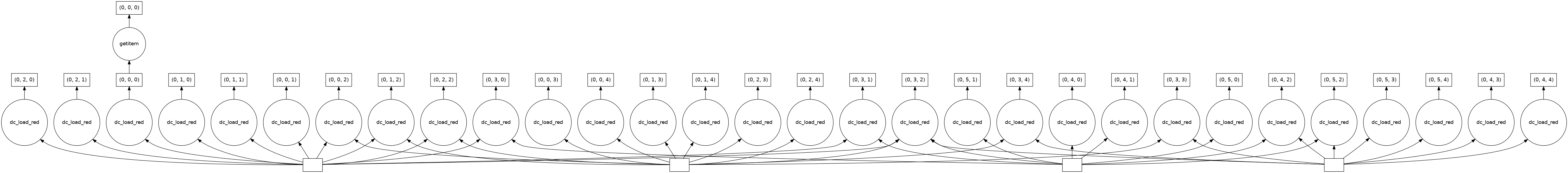
Task graphs
When using lazy-loading, Dask breaks up the loading operation into a series of steps. A useful way to visualise the steps is the task graph, which can be accessed by adding the .visualize() .data
The task graph is read from bottom to top.
The four rectangles at the bottom of the graph are the database entries representing the files that need to be read to load the data.
Above the rectangles are individual load commands (in the circles) that will do the reading. There is one for each chunk. The arrows describe which files need to be read for each operation: the chunk on the left needs data from all four database entries, whereas the chunk on the right only needs data from one.
At the very top are the indexes of the chunks that will make up the final array.
Adding more tasks
The power of this method comes from chaining tasks together before loading the data. This is because Dask will only load the data that is required by the final operation in the chain.
We can demonstrate this by requesting only a small portion of the red band. If we do this for the lazy-loaded data, we can view the new task graph:
Notice that the new task getitem .load() extract_from_red
We can establish that the above operation yields the same result as loading the data without Dask and subsetting it by running the command below:
The loaded arrays match: True
Since the arrays are the same, it is worth using lazy-loading to chain operations together, then calling .load() red data red green blue red
Multiple tasks
The power of using lazy-loading in Dask is that you can continue to chain operations together until you are ready to get the answer.
Here, we chain multiple steps together to calculate a new band for our array. Specifically, we use the red nir
Doing this adds the new ndvi lazy_data
<xarray.Dataset>
Dimensions:      (time: 1, y: 17925, x: 14473)
Coordinates:
  * time         (time) datetime64[ns] 2018-07-02T11:59:59.999999
  * y            (y) float64 -2.501e+06 -2.501e+06 ... -2.681e+06 -2.681e+06
  * x            (x) float64 2.316e+06 2.316e+06 2.316e+06 ... 2.46e+06 2.46e+06
    spatial_ref  int32 6933
Data variables:
    red          (time, y, x) uint16 dask.array<chunksize=(1, 3000, 3000), meta=np.ndarray>
    green        (time, y, x) uint16 dask.array<chunksize=(1, 3000, 3000), meta=np.ndarray>
    blue         (time, y, x) uint16 dask.array<chunksize=(1, 3000, 3000), meta=np.ndarray>
    nir          (time, y, x) uint16 dask.array<chunksize=(1, 3000, 3000), meta=np.ndarray>
    ndvi         (time, y, x) float64 dask.array<chunksize=(1, 3000, 3000), meta=np.ndarray>
Attributes:
    crs:           epsg:6933
grid_mapping: spatial_ref Dimensions:
Coordinates: (4)
time
(time)
datetime64[ns]
2018-07-02T11:59:59.999999
units : seconds since 1970-01-01 00:00:00 array(['2018-07-02T11:59:59.999999000'], dtype='datetime64[ns]') y
(y)
float64
-2.501e+06 ... -2.681e+06
units : metre resolution : -10.0 crs : epsg:6933 array([-2501275., -2501285., -2501295., ..., -2680495., -2680505., -2680515.]) x
(x)
float64
2.316e+06 2.316e+06 ... 2.46e+06
units : metre resolution : 10.0 crs : epsg:6933 array([2315675., 2315685., 2315695., ..., 2460375., 2460385., 2460395.]) spatial_ref
()
int32
6933
spatial_ref : PROJCS["WGS 84 / NSIDC EASE-Grid 2.0 Global",GEOGCS["WGS 84",DATUM["WGS_1984",SPHEROID["WGS 84",6378137,298.257223563,AUTHORITY["EPSG","7030"]],AUTHORITY["EPSG","6326"]],PRIMEM["Greenwich",0,AUTHORITY["EPSG","8901"]],UNIT["degree",0.0174532925199433,AUTHORITY["EPSG","9122"]],AUTHORITY["EPSG","4326"]],PROJECTION["Cylindrical_Equal_Area"],PARAMETER["standard_parallel_1",30],PARAMETER["central_meridian",0],PARAMETER["false_easting",0],PARAMETER["false_northing",0],UNIT["metre",1,AUTHORITY["EPSG","9001"]],AXIS["Easting",EAST],AXIS["Northing",NORTH],AUTHORITY["EPSG","6933"]] grid_mapping_name : lambert_cylindrical_equal_area Data variables: (5)
red
(time, y, x)
uint16
dask.array<chunksize=(1, 3000, 3000), meta=np.ndarray>
units : 1 nodata : 0 crs : epsg:6933 grid_mapping : spatial_ref
Array
Chunk
Bytes
494.82 MiB
17.17 MiB
Shape
(1, 17925, 14473)
(1, 3000, 3000)
Dask graph
30 chunks in 1 graph layer
Data type
uint16 numpy.ndarray
14473
17925
1
green
(time, y, x)
uint16
dask.array<chunksize=(1, 3000, 3000), meta=np.ndarray>
units : 1 nodata : 0 crs : epsg:6933 grid_mapping : spatial_ref
Array
Chunk
Bytes
494.82 MiB
17.17 MiB
Shape
(1, 17925, 14473)
(1, 3000, 3000)
Dask graph
30 chunks in 1 graph layer
Data type
uint16 numpy.ndarray
14473
17925
1
blue
(time, y, x)
uint16
dask.array<chunksize=(1, 3000, 3000), meta=np.ndarray>
units : 1 nodata : 0 crs : epsg:6933 grid_mapping : spatial_ref
Array
Chunk
Bytes
494.82 MiB
17.17 MiB
Shape
(1, 17925, 14473)
(1, 3000, 3000)
Dask graph
30 chunks in 1 graph layer
Data type
uint16 numpy.ndarray
14473
17925
1
nir
(time, y, x)
uint16
dask.array<chunksize=(1, 3000, 3000), meta=np.ndarray>
units : 1 nodata : 0 crs : epsg:6933 grid_mapping : spatial_ref
Array
Chunk
Bytes
494.82 MiB
17.17 MiB
Shape
(1, 17925, 14473)
(1, 3000, 3000)
Dask graph
30 chunks in 1 graph layer
Data type
uint16 numpy.ndarray
14473
17925
1
ndvi
(time, y, x)
float64
dask.array<chunksize=(1, 3000, 3000), meta=np.ndarray>
Array
Chunk
Bytes
1.93 GiB
68.66 MiB
Shape
(1, 17925, 14473)
(1, 3000, 3000)
Dask graph
30 chunks in 5 graph layers
Data type
float64 numpy.ndarray
14473
17925
1
Indexes: (3)
PandasIndex
PandasIndex(DatetimeIndex(['2018-07-02 11:59:59.999999'], dtype='datetime64[ns]', name='time', freq=None)) PandasIndex
PandasIndex(Index([-2501275.0, -2501285.0, -2501295.0, -2501305.0, -2501315.0, -2501325.0,
       -2501335.0, -2501345.0, -2501355.0, -2501365.0,
       ...
       -2680425.0, -2680435.0, -2680445.0, -2680455.0, -2680465.0, -2680475.0,
       -2680485.0, -2680495.0, -2680505.0, -2680515.0],
dtype='float64', name='y', length=17925)) PandasIndex
PandasIndex(Index([2315675.0, 2315685.0, 2315695.0, 2315705.0, 2315715.0, 2315725.0,
       2315735.0, 2315745.0, 2315755.0, 2315765.0,
       ...
       2460305.0, 2460315.0, 2460325.0, 2460335.0, 2460345.0, 2460355.0,
       2460365.0, 2460375.0, 2460385.0, 2460395.0],
      dtype='float64', name='x', length=14473))
Attributes: (2)
crs : epsg:6933 grid_mapping : spatial_ref
Now that the operation is defined, we can view its task graph:
Reading the graph bottom-to-top, we can see the equation taking place. The add sub
We can see how each output chunk is independent from the others. This means we could calculate each chunk without ever having to load all of the bands into memory at the same time.
Finally, we can calculate the NDVI values by calling the .load() ndvi_load
/usr/local/lib/python3.10/dist-packages/dask/core.py:119: RuntimeWarning: invalid value encountered in divide
  return func(*(_execute_task(a, cache) for a in args))
<xarray.DataArray 'ndvi' (time: 1, y: 17925, x: 14473)>
array([[[0.34023759, 0.33039389, 0.32077593, ..., 0.37083061,
         0.38180611, 0.37719008],
        [0.33235381, 0.33006912, 0.32352124, ..., 0.36498708,
         0.36280884, 0.38525155],
        [0.31681217, 0.3295325 , 0.32962448, ..., 0.36790286,
         0.35850274, 0.36588629],
        ...,
        [0.19612476, 0.1977664 , 0.20513408, ..., 0.23719165,
         0.26922088, 0.2815534 ],
        [0.19981128, 0.20527046, 0.20905764, ..., 0.2352666 ,
         0.25160983, 0.2643065 ],
        [0.20236407, 0.20495443, 0.20352341, ..., 0.23283311,
         0.25068493, 0.25750174]]])
Coordinates:
  * time         (time) datetime64[ns] 2018-07-02T11:59:59.999999
  * y            (y) float64 -2.501e+06 -2.501e+06 ... -2.681e+06 -2.681e+06
  * x            (x) float64 2.316e+06 2.316e+06 2.316e+06 ... 2.46e+06 2.46e+06
spatial_ref int32 6933 0.3402 0.3304 0.3208 0.3209 0.3217 ... 0.2427 0.2328 0.2507 0.2575
array([[[0.34023759, 0.33039389, 0.32077593, ..., 0.37083061,
         0.38180611, 0.37719008],
        [0.33235381, 0.33006912, 0.32352124, ..., 0.36498708,
         0.36280884, 0.38525155],
        [0.31681217, 0.3295325 , 0.32962448, ..., 0.36790286,
         0.35850274, 0.36588629],
        ...,
        [0.19612476, 0.1977664 , 0.20513408, ..., 0.23719165,
         0.26922088, 0.2815534 ],
        [0.19981128, 0.20527046, 0.20905764, ..., 0.2352666 ,
         0.25160983, 0.2643065 ],
        [0.20236407, 0.20495443, 0.20352341, ..., 0.23283311,
         0.25068493, 0.25750174]]])
Coordinates: (4)
time
(time)
datetime64[ns]
2018-07-02T11:59:59.999999
units : seconds since 1970-01-01 00:00:00 array(['2018-07-02T11:59:59.999999000'], dtype='datetime64[ns]') y
(y)
float64
-2.501e+06 ... -2.681e+06
units : metre resolution : -10.0 crs : epsg:6933 array([-2501275., -2501285., -2501295., ..., -2680495., -2680505., -2680515.]) x
(x)
float64
2.316e+06 2.316e+06 ... 2.46e+06
units : metre resolution : 10.0 crs : epsg:6933 array([2315675., 2315685., 2315695., ..., 2460375., 2460385., 2460395.]) spatial_ref
()
int32
6933
spatial_ref : PROJCS["WGS 84 / NSIDC EASE-Grid 2.0 Global",GEOGCS["WGS 84",DATUM["WGS_1984",SPHEROID["WGS 84",6378137,298.257223563,AUTHORITY["EPSG","7030"]],AUTHORITY["EPSG","6326"]],PRIMEM["Greenwich",0,AUTHORITY["EPSG","8901"]],UNIT["degree",0.0174532925199433,AUTHORITY["EPSG","9122"]],AUTHORITY["EPSG","4326"]],PROJECTION["Cylindrical_Equal_Area"],PARAMETER["standard_parallel_1",30],PARAMETER["central_meridian",0],PARAMETER["false_easting",0],PARAMETER["false_northing",0],UNIT["metre",1,AUTHORITY["EPSG","9001"]],AXIS["Easting",EAST],AXIS["Northing",NORTH],AUTHORITY["EPSG","6933"]] grid_mapping_name : lambert_cylindrical_equal_area Indexes: (3)
PandasIndex
PandasIndex(DatetimeIndex(['2018-07-02 11:59:59.999999'], dtype='datetime64[ns]', name='time', freq=None)) PandasIndex
PandasIndex(Index([-2501275.0, -2501285.0, -2501295.0, -2501305.0, -2501315.0, -2501325.0,
       -2501335.0, -2501345.0, -2501355.0, -2501365.0,
       ...
       -2680425.0, -2680435.0, -2680445.0, -2680455.0, -2680465.0, -2680475.0,
       -2680485.0, -2680495.0, -2680505.0, -2680515.0],
dtype='float64', name='y', length=17925)) PandasIndex
PandasIndex(Index([2315675.0, 2315685.0, 2315695.0, 2315705.0, 2315715.0, 2315725.0,
       2315735.0, 2315745.0, 2315755.0, 2315765.0,
       ...
       2460305.0, 2460315.0, 2460325.0, 2460335.0, 2460345.0, 2460355.0,
       2460365.0, 2460375.0, 2460385.0, 2460395.0],
      dtype='float64', name='x', length=14473))
Attributes: (0)
Note that running the .load() ndvi lazy_load
<xarray.Dataset>
Dimensions:      (time: 1, y: 17925, x: 14473)
Coordinates:
  * time         (time) datetime64[ns] 2018-07-02T11:59:59.999999
  * y            (y) float64 -2.501e+06 -2.501e+06 ... -2.681e+06 -2.681e+06
  * x            (x) float64 2.316e+06 2.316e+06 2.316e+06 ... 2.46e+06 2.46e+06
    spatial_ref  int32 6933
Data variables:
    red          (time, y, x) uint16 dask.array<chunksize=(1, 3000, 3000), meta=np.ndarray>
    green        (time, y, x) uint16 dask.array<chunksize=(1, 3000, 3000), meta=np.ndarray>
    blue         (time, y, x) uint16 dask.array<chunksize=(1, 3000, 3000), meta=np.ndarray>
    nir          (time, y, x) uint16 dask.array<chunksize=(1, 3000, 3000), meta=np.ndarray>
    ndvi         (time, y, x) float64 0.3402 0.3304 0.3208 ... 0.2507 0.2575
Attributes:
    crs:           epsg:6933
grid_mapping: spatial_ref Dimensions:
Coordinates: (4)
time
(time)
datetime64[ns]
2018-07-02T11:59:59.999999
units : seconds since 1970-01-01 00:00:00 array(['2018-07-02T11:59:59.999999000'], dtype='datetime64[ns]') y
(y)
float64
-2.501e+06 ... -2.681e+06
units : metre resolution : -10.0 crs : epsg:6933 array([-2501275., -2501285., -2501295., ..., -2680495., -2680505., -2680515.]) x
(x)
float64
2.316e+06 2.316e+06 ... 2.46e+06
units : metre resolution : 10.0 crs : epsg:6933 array([2315675., 2315685., 2315695., ..., 2460375., 2460385., 2460395.]) spatial_ref
()
int32
6933
spatial_ref : PROJCS["WGS 84 / NSIDC EASE-Grid 2.0 Global",GEOGCS["WGS 84",DATUM["WGS_1984",SPHEROID["WGS 84",6378137,298.257223563,AUTHORITY["EPSG","7030"]],AUTHORITY["EPSG","6326"]],PRIMEM["Greenwich",0,AUTHORITY["EPSG","8901"]],UNIT["degree",0.0174532925199433,AUTHORITY["EPSG","9122"]],AUTHORITY["EPSG","4326"]],PROJECTION["Cylindrical_Equal_Area"],PARAMETER["standard_parallel_1",30],PARAMETER["central_meridian",0],PARAMETER["false_easting",0],PARAMETER["false_northing",0],UNIT["metre",1,AUTHORITY["EPSG","9001"]],AXIS["Easting",EAST],AXIS["Northing",NORTH],AUTHORITY["EPSG","6933"]] grid_mapping_name : lambert_cylindrical_equal_area Data variables: (5)
red
(time, y, x)
uint16
dask.array<chunksize=(1, 3000, 3000), meta=np.ndarray>
units : 1 nodata : 0 crs : epsg:6933 grid_mapping : spatial_ref
Array
Chunk
Bytes
494.82 MiB
17.17 MiB
Shape
(1, 17925, 14473)
(1, 3000, 3000)
Dask graph
30 chunks in 1 graph layer
Data type
uint16 numpy.ndarray
14473
17925
1
green
(time, y, x)
uint16
dask.array<chunksize=(1, 3000, 3000), meta=np.ndarray>
units : 1 nodata : 0 crs : epsg:6933 grid_mapping : spatial_ref
Array
Chunk
Bytes
494.82 MiB
17.17 MiB
Shape
(1, 17925, 14473)
(1, 3000, 3000)
Dask graph
30 chunks in 1 graph layer
Data type
uint16 numpy.ndarray
14473
17925
1
blue
(time, y, x)
uint16
dask.array<chunksize=(1, 3000, 3000), meta=np.ndarray>
units : 1 nodata : 0 crs : epsg:6933 grid_mapping : spatial_ref
Array
Chunk
Bytes
494.82 MiB
17.17 MiB
Shape
(1, 17925, 14473)
(1, 3000, 3000)
Dask graph
30 chunks in 1 graph layer
Data type
uint16 numpy.ndarray
14473
17925
1
nir
(time, y, x)
uint16
dask.array<chunksize=(1, 3000, 3000), meta=np.ndarray>
units : 1 nodata : 0 crs : epsg:6933 grid_mapping : spatial_ref
Array
Chunk
Bytes
494.82 MiB
17.17 MiB
Shape
(1, 17925, 14473)
(1, 3000, 3000)
Dask graph
30 chunks in 1 graph layer
Data type
uint16 numpy.ndarray
14473
17925
1
ndvi
(time, y, x)
float64
0.3402 0.3304 ... 0.2507 0.2575
array([[[0.34023759, 0.33039389, 0.32077593, ..., 0.37083061,
         0.38180611, 0.37719008],
        [0.33235381, 0.33006912, 0.32352124, ..., 0.36498708,
         0.36280884, 0.38525155],
        [0.31681217, 0.3295325 , 0.32962448, ..., 0.36790286,
         0.35850274, 0.36588629],
        ...,
        [0.19612476, 0.1977664 , 0.20513408, ..., 0.23719165,
         0.26922088, 0.2815534 ],
        [0.19981128, 0.20527046, 0.20905764, ..., 0.2352666 ,
         0.25160983, 0.2643065 ],
        [0.20236407, 0.20495443, 0.20352341, ..., 0.23283311,
         0.25068493, 0.25750174]]])
Indexes: (3)
PandasIndex
PandasIndex(DatetimeIndex(['2018-07-02 11:59:59.999999'], dtype='datetime64[ns]', name='time', freq=None)) PandasIndex
PandasIndex(Index([-2501275.0, -2501285.0, -2501295.0, -2501305.0, -2501315.0, -2501325.0,
       -2501335.0, -2501345.0, -2501355.0, -2501365.0,
       ...
       -2680425.0, -2680435.0, -2680445.0, -2680455.0, -2680465.0, -2680475.0,
       -2680485.0, -2680495.0, -2680505.0, -2680515.0],
dtype='float64', name='y', length=17925)) PandasIndex
PandasIndex(Index([2315675.0, 2315685.0, 2315695.0, 2315705.0, 2315715.0, 2315725.0,
       2315735.0, 2315745.0, 2315755.0, 2315765.0,
       ...
       2460305.0, 2460315.0, 2460325.0, 2460335.0, 2460345.0, 2460355.0,
       2460365.0, 2460375.0, 2460385.0, 2460395.0],
      dtype='float64', name='x', length=14473))
Attributes: (2)
crs : epsg:6933 grid_mapping : spatial_ref
You can see that ndvi
Keeping variables as Dask arrays
If you wanted to calculate the NDVI values, but leave ndvi lazy_load .compute()
To demonstrate this, we first redefine the ndvi
<xarray.Dataset>
Dimensions:      (time: 1, y: 17925, x: 14473)
Coordinates:
  * time         (time) datetime64[ns] 2018-07-02T11:59:59.999999
  * y            (y) float64 -2.501e+06 -2.501e+06 ... -2.681e+06 -2.681e+06
  * x            (x) float64 2.316e+06 2.316e+06 2.316e+06 ... 2.46e+06 2.46e+06
    spatial_ref  int32 6933
Data variables:
    red          (time, y, x) uint16 dask.array<chunksize=(1, 3000, 3000), meta=np.ndarray>
    green        (time, y, x) uint16 dask.array<chunksize=(1, 3000, 3000), meta=np.ndarray>
    blue         (time, y, x) uint16 dask.array<chunksize=(1, 3000, 3000), meta=np.ndarray>
    nir          (time, y, x) uint16 dask.array<chunksize=(1, 3000, 3000), meta=np.ndarray>
    ndvi         (time, y, x) float64 dask.array<chunksize=(1, 3000, 3000), meta=np.ndarray>
Attributes:
    crs:           epsg:6933
grid_mapping: spatial_ref Dimensions:
Coordinates: (4)
time
(time)
datetime64[ns]
2018-07-02T11:59:59.999999
units : seconds since 1970-01-01 00:00:00 array(['2018-07-02T11:59:59.999999000'], dtype='datetime64[ns]') y
(y)
float64
-2.501e+06 ... -2.681e+06
units : metre resolution : -10.0 crs : epsg:6933 array([-2501275., -2501285., -2501295., ..., -2680495., -2680505., -2680515.]) x
(x)
float64
2.316e+06 2.316e+06 ... 2.46e+06
units : metre resolution : 10.0 crs : epsg:6933 array([2315675., 2315685., 2315695., ..., 2460375., 2460385., 2460395.]) spatial_ref
()
int32
6933
spatial_ref : PROJCS["WGS 84 / NSIDC EASE-Grid 2.0 Global",GEOGCS["WGS 84",DATUM["WGS_1984",SPHEROID["WGS 84",6378137,298.257223563,AUTHORITY["EPSG","7030"]],AUTHORITY["EPSG","6326"]],PRIMEM["Greenwich",0,AUTHORITY["EPSG","8901"]],UNIT["degree",0.0174532925199433,AUTHORITY["EPSG","9122"]],AUTHORITY["EPSG","4326"]],PROJECTION["Cylindrical_Equal_Area"],PARAMETER["standard_parallel_1",30],PARAMETER["central_meridian",0],PARAMETER["false_easting",0],PARAMETER["false_northing",0],UNIT["metre",1,AUTHORITY["EPSG","9001"]],AXIS["Easting",EAST],AXIS["Northing",NORTH],AUTHORITY["EPSG","6933"]] grid_mapping_name : lambert_cylindrical_equal_area Data variables: (5)
red
(time, y, x)
uint16
dask.array<chunksize=(1, 3000, 3000), meta=np.ndarray>
units : 1 nodata : 0 crs : epsg:6933 grid_mapping : spatial_ref
Array
Chunk
Bytes
494.82 MiB
17.17 MiB
Shape
(1, 17925, 14473)
(1, 3000, 3000)
Dask graph
30 chunks in 1 graph layer
Data type
uint16 numpy.ndarray
14473
17925
1
green
(time, y, x)
uint16
dask.array<chunksize=(1, 3000, 3000), meta=np.ndarray>
units : 1 nodata : 0 crs : epsg:6933 grid_mapping : spatial_ref
Array
Chunk
Bytes
494.82 MiB
17.17 MiB
Shape
(1, 17925, 14473)
(1, 3000, 3000)
Dask graph
30 chunks in 1 graph layer
Data type
uint16 numpy.ndarray
14473
17925
1
blue
(time, y, x)
uint16
dask.array<chunksize=(1, 3000, 3000), meta=np.ndarray>
units : 1 nodata : 0 crs : epsg:6933 grid_mapping : spatial_ref
Array
Chunk
Bytes
494.82 MiB
17.17 MiB
Shape
(1, 17925, 14473)
(1, 3000, 3000)
Dask graph
30 chunks in 1 graph layer
Data type
uint16 numpy.ndarray
14473
17925
1
nir
(time, y, x)
uint16
dask.array<chunksize=(1, 3000, 3000), meta=np.ndarray>
units : 1 nodata : 0 crs : epsg:6933 grid_mapping : spatial_ref
Array
Chunk
Bytes
494.82 MiB
17.17 MiB
Shape
(1, 17925, 14473)
(1, 3000, 3000)
Dask graph
30 chunks in 1 graph layer
Data type
uint16 numpy.ndarray
14473
17925
1
ndvi
(time, y, x)
float64
dask.array<chunksize=(1, 3000, 3000), meta=np.ndarray>
Array
Chunk
Bytes
1.93 GiB
68.66 MiB
Shape
(1, 17925, 14473)
(1, 3000, 3000)
Dask graph
30 chunks in 5 graph layers
Data type
float64 numpy.ndarray
14473
17925
1
Indexes: (3)
PandasIndex
PandasIndex(DatetimeIndex(['2018-07-02 11:59:59.999999'], dtype='datetime64[ns]', name='time', freq=None)) PandasIndex
PandasIndex(Index([-2501275.0, -2501285.0, -2501295.0, -2501305.0, -2501315.0, -2501325.0,
       -2501335.0, -2501345.0, -2501355.0, -2501365.0,
       ...
       -2680425.0, -2680435.0, -2680445.0, -2680455.0, -2680465.0, -2680475.0,
       -2680485.0, -2680495.0, -2680505.0, -2680515.0],
dtype='float64', name='y', length=17925)) PandasIndex
PandasIndex(Index([2315675.0, 2315685.0, 2315695.0, 2315705.0, 2315715.0, 2315725.0,
       2315735.0, 2315745.0, 2315755.0, 2315765.0,
       ...
       2460305.0, 2460315.0, 2460325.0, 2460335.0, 2460345.0, 2460355.0,
       2460365.0, 2460375.0, 2460385.0, 2460395.0],
      dtype='float64', name='x', length=14473))
Attributes: (2)
crs : epsg:6933 grid_mapping : spatial_ref
Now, we perform the same steps as before to calculate NDVI, but use .compute() .load():
<xarray.DataArray 'ndvi' (time: 1, y: 17925, x: 14473)>
array([[[0.34023759, 0.33039389, 0.32077593, ..., 0.37083061,
         0.38180611, 0.37719008],
        [0.33235381, 0.33006912, 0.32352124, ..., 0.36498708,
         0.36280884, 0.38525155],
        [0.31681217, 0.3295325 , 0.32962448, ..., 0.36790286,
         0.35850274, 0.36588629],
        ...,
        [0.19612476, 0.1977664 , 0.20513408, ..., 0.23719165,
         0.26922088, 0.2815534 ],
        [0.19981128, 0.20527046, 0.20905764, ..., 0.2352666 ,
         0.25160983, 0.2643065 ],
        [0.20236407, 0.20495443, 0.20352341, ..., 0.23283311,
         0.25068493, 0.25750174]]])
Coordinates:
  * time         (time) datetime64[ns] 2018-07-02T11:59:59.999999
  * y            (y) float64 -2.501e+06 -2.501e+06 ... -2.681e+06 -2.681e+06
  * x            (x) float64 2.316e+06 2.316e+06 2.316e+06 ... 2.46e+06 2.46e+06
spatial_ref int32 6933 0.3402 0.3304 0.3208 0.3209 0.3217 ... 0.2427 0.2328 0.2507 0.2575
array([[[0.34023759, 0.33039389, 0.32077593, ..., 0.37083061,
         0.38180611, 0.37719008],
        [0.33235381, 0.33006912, 0.32352124, ..., 0.36498708,
         0.36280884, 0.38525155],
        [0.31681217, 0.3295325 , 0.32962448, ..., 0.36790286,
         0.35850274, 0.36588629],
        ...,
        [0.19612476, 0.1977664 , 0.20513408, ..., 0.23719165,
         0.26922088, 0.2815534 ],
        [0.19981128, 0.20527046, 0.20905764, ..., 0.2352666 ,
         0.25160983, 0.2643065 ],
        [0.20236407, 0.20495443, 0.20352341, ..., 0.23283311,
         0.25068493, 0.25750174]]])
Coordinates: (4)
time
(time)
datetime64[ns]
2018-07-02T11:59:59.999999
units : seconds since 1970-01-01 00:00:00 array(['2018-07-02T11:59:59.999999000'], dtype='datetime64[ns]') y
(y)
float64
-2.501e+06 ... -2.681e+06
units : metre resolution : -10.0 crs : epsg:6933 array([-2501275., -2501285., -2501295., ..., -2680495., -2680505., -2680515.]) x
(x)
float64
2.316e+06 2.316e+06 ... 2.46e+06
units : metre resolution : 10.0 crs : epsg:6933 array([2315675., 2315685., 2315695., ..., 2460375., 2460385., 2460395.]) spatial_ref
()
int32
6933
spatial_ref : PROJCS["WGS 84 / NSIDC EASE-Grid 2.0 Global",GEOGCS["WGS 84",DATUM["WGS_1984",SPHEROID["WGS 84",6378137,298.257223563,AUTHORITY["EPSG","7030"]],AUTHORITY["EPSG","6326"]],PRIMEM["Greenwich",0,AUTHORITY["EPSG","8901"]],UNIT["degree",0.0174532925199433,AUTHORITY["EPSG","9122"]],AUTHORITY["EPSG","4326"]],PROJECTION["Cylindrical_Equal_Area"],PARAMETER["standard_parallel_1",30],PARAMETER["central_meridian",0],PARAMETER["false_easting",0],PARAMETER["false_northing",0],UNIT["metre",1,AUTHORITY["EPSG","9001"]],AXIS["Easting",EAST],AXIS["Northing",NORTH],AUTHORITY["EPSG","6933"]] grid_mapping_name : lambert_cylindrical_equal_area Indexes: (3)
PandasIndex
PandasIndex(DatetimeIndex(['2018-07-02 11:59:59.999999'], dtype='datetime64[ns]', name='time', freq=None)) PandasIndex
PandasIndex(Index([-2501275.0, -2501285.0, -2501295.0, -2501305.0, -2501315.0, -2501325.0,
       -2501335.0, -2501345.0, -2501355.0, -2501365.0,
       ...
       -2680425.0, -2680435.0, -2680445.0, -2680455.0, -2680465.0, -2680475.0,
       -2680485.0, -2680495.0, -2680505.0, -2680515.0],
dtype='float64', name='y', length=17925)) PandasIndex
PandasIndex(Index([2315675.0, 2315685.0, 2315695.0, 2315705.0, 2315715.0, 2315725.0,
       2315735.0, 2315745.0, 2315755.0, 2315765.0,
       ...
       2460305.0, 2460315.0, 2460325.0, 2460335.0, 2460345.0, 2460355.0,
       2460365.0, 2460375.0, 2460385.0, 2460395.0],
      dtype='float64', name='x', length=14473))
Attributes: (0)
You can see that the values have been calculated, but as shown below, the ndvi
<xarray.Dataset>
Dimensions:      (time: 1, y: 17925, x: 14473)
Coordinates:
  * time         (time) datetime64[ns] 2018-07-02T11:59:59.999999
  * y            (y) float64 -2.501e+06 -2.501e+06 ... -2.681e+06 -2.681e+06
  * x            (x) float64 2.316e+06 2.316e+06 2.316e+06 ... 2.46e+06 2.46e+06
    spatial_ref  int32 6933
Data variables:
    red          (time, y, x) uint16 dask.array<chunksize=(1, 3000, 3000), meta=np.ndarray>
    green        (time, y, x) uint16 dask.array<chunksize=(1, 3000, 3000), meta=np.ndarray>
    blue         (time, y, x) uint16 dask.array<chunksize=(1, 3000, 3000), meta=np.ndarray>
    nir          (time, y, x) uint16 dask.array<chunksize=(1, 3000, 3000), meta=np.ndarray>
    ndvi         (time, y, x) float64 dask.array<chunksize=(1, 3000, 3000), meta=np.ndarray>
Attributes:
    crs:           epsg:6933
grid_mapping: spatial_ref Dimensions:
Coordinates: (4)
time
(time)
datetime64[ns]
2018-07-02T11:59:59.999999
units : seconds since 1970-01-01 00:00:00 array(['2018-07-02T11:59:59.999999000'], dtype='datetime64[ns]') y
(y)
float64
-2.501e+06 ... -2.681e+06
units : metre resolution : -10.0 crs : epsg:6933 array([-2501275., -2501285., -2501295., ..., -2680495., -2680505., -2680515.]) x
(x)
float64
2.316e+06 2.316e+06 ... 2.46e+06
units : metre resolution : 10.0 crs : epsg:6933 array([2315675., 2315685., 2315695., ..., 2460375., 2460385., 2460395.]) spatial_ref
()
int32
6933
spatial_ref : PROJCS["WGS 84 / NSIDC EASE-Grid 2.0 Global",GEOGCS["WGS 84",DATUM["WGS_1984",SPHEROID["WGS 84",6378137,298.257223563,AUTHORITY["EPSG","7030"]],AUTHORITY["EPSG","6326"]],PRIMEM["Greenwich",0,AUTHORITY["EPSG","8901"]],UNIT["degree",0.0174532925199433,AUTHORITY["EPSG","9122"]],AUTHORITY["EPSG","4326"]],PROJECTION["Cylindrical_Equal_Area"],PARAMETER["standard_parallel_1",30],PARAMETER["central_meridian",0],PARAMETER["false_easting",0],PARAMETER["false_northing",0],UNIT["metre",1,AUTHORITY["EPSG","9001"]],AXIS["Easting",EAST],AXIS["Northing",NORTH],AUTHORITY["EPSG","6933"]] grid_mapping_name : lambert_cylindrical_equal_area Data variables: (5)
red
(time, y, x)
uint16
dask.array<chunksize=(1, 3000, 3000), meta=np.ndarray>
units : 1 nodata : 0 crs : epsg:6933 grid_mapping : spatial_ref
Array
Chunk
Bytes
494.82 MiB
17.17 MiB
Shape
(1, 17925, 14473)
(1, 3000, 3000)
Dask graph
30 chunks in 1 graph layer
Data type
uint16 numpy.ndarray
14473
17925
1
green
(time, y, x)
uint16
dask.array<chunksize=(1, 3000, 3000), meta=np.ndarray>
units : 1 nodata : 0 crs : epsg:6933 grid_mapping : spatial_ref
Array
Chunk
Bytes
494.82 MiB
17.17 MiB
Shape
(1, 17925, 14473)
(1, 3000, 3000)
Dask graph
30 chunks in 1 graph layer
Data type
uint16 numpy.ndarray
14473
17925
1
blue
(time, y, x)
uint16
dask.array<chunksize=(1, 3000, 3000), meta=np.ndarray>
units : 1 nodata : 0 crs : epsg:6933 grid_mapping : spatial_ref
Array
Chunk
Bytes
494.82 MiB
17.17 MiB
Shape
(1, 17925, 14473)
(1, 3000, 3000)
Dask graph
30 chunks in 1 graph layer
Data type
uint16 numpy.ndarray
14473
17925
1
nir
(time, y, x)
uint16
dask.array<chunksize=(1, 3000, 3000), meta=np.ndarray>
units : 1 nodata : 0 crs : epsg:6933 grid_mapping : spatial_ref
Array
Chunk
Bytes
494.82 MiB
17.17 MiB
Shape
(1, 17925, 14473)
(1, 3000, 3000)
Dask graph
30 chunks in 1 graph layer
Data type
uint16 numpy.ndarray
14473
17925
1
ndvi
(time, y, x)
float64
dask.array<chunksize=(1, 3000, 3000), meta=np.ndarray>
Array
Chunk
Bytes
1.93 GiB
68.66 MiB
Shape
(1, 17925, 14473)
(1, 3000, 3000)
Dask graph
30 chunks in 5 graph layers
Data type
float64 numpy.ndarray
14473
17925
1
Indexes: (3)
PandasIndex
PandasIndex(DatetimeIndex(['2018-07-02 11:59:59.999999'], dtype='datetime64[ns]', name='time', freq=None)) PandasIndex
PandasIndex(Index([-2501275.0, -2501285.0, -2501295.0, -2501305.0, -2501315.0, -2501325.0,
       -2501335.0, -2501345.0, -2501355.0, -2501365.0,
       ...
       -2680425.0, -2680435.0, -2680445.0, -2680455.0, -2680465.0, -2680475.0,
       -2680485.0, -2680495.0, -2680505.0, -2680515.0],
dtype='float64', name='y', length=17925)) PandasIndex
PandasIndex(Index([2315675.0, 2315685.0, 2315695.0, 2315705.0, 2315715.0, 2315725.0,
       2315735.0, 2315745.0, 2315755.0, 2315765.0,
       ...
       2460305.0, 2460315.0, 2460325.0, 2460335.0, 2460345.0, 2460355.0,
       2460365.0, 2460375.0, 2460385.0, 2460395.0],
      dtype='float64', name='x', length=14473))
Attributes: (2)
crs : epsg:6933 grid_mapping : spatial_ref
Using .compute() .compute()
Further Resources
For further reading on how Dask works, and how it is used by xarray, see these resources:
Other notebooks
This is the last notebook in the beginner’s guide; if anything was unclear, we recommend revising the relevant notebook:
Jupyter Notebooks
Products and Measurements
Loading data
Plotting
Performing a basic analysis
Introduction to numpy
Introduction to xarray
Parallel processing with Dask (this notebook)
Once you have completed the above eight tutorials, join advanced users in exploring:
The “Datasets” directory in the repository, where you can explore DE Africa products in depth.
The “Frequently used code” directory, which contains a recipe book of common techniques and methods for analysing DE Africa data.
The “Real-world examples” directory, which provides more complex workflows and analysis case studies.