Introduction à xarray
Prérequis : Les utilisateurs de ce notebook doivent avoir une compréhension de base de :
Comment exécuter un Jupyter notebook
Comment travailler avec numpy
Mots-clés guide du débutant; xarray, package python; xarray
Aperçu
Xarray est une bibliothèque Python qui simplifie le travail avec des tableaux multidimensionnels étiquetés. Xarray introduit des étiquettes sous forme de dimensions, de coordonnées et d’attributs sur des tableaux numpy bruts, permettant un développement plus intuitif et concis. Vous trouverez plus d’informations sur les structures de données et les fonctions xarray ici <http://xarray.pydata.org/en/stable/>`__.
Une fois que vous avez terminé ce bloc-notes, vous souhaiterez peut-être améliorer davantage vos compétences en matière de xarray. Ce « bloc-notes externe <https://rabernat.github.io/research_computing/xarray.html> »__ présente d’autres utilisations de xarray et peut vous aider à améliorer davantage vos compétences.
Description
Ce notebook est conçu pour présenter aux utilisateurs « xarray » à l’aide de code Python dans Jupyter Notebooks via JupyterLab.
Les sujets abordés comprennent :
Comment utiliser les fonctions xarray dans une cellule Jupyter Notebook
Comment accéder aux dimensions et aux métadonnées du xarray
Utilisation de l’indexation pour explorer les données multidimensionnelles de matrice X
Application des fonctions intégrées de xarray telles que la somme, l’écart type et la moyenne
Commencer
Pour exécuter ce bloc-notes, exécutez toutes les cellules du bloc-notes en commençant par la cellule « Charger les packages ». Pour obtenir de l’aide sur l’exécution des cellules du bloc-notes, reportez-vous au bloc-notes Jupyter Notebooks <01_Jupyter_notebooks.ipynb>`__.
Charger des paquets
[1]:
%matplotlib inline
import matplotlib.pyplot as plt
import numpy as np
import xarray as xr
Introduction à xarray
DE Africa utilise xarray comme modèle de données principal. Pour mieux comprendre de quoi il s’agit, commençons par une expérience simple en utilisant une combinaison de tableaux numpy simples et de dictionnaires Python.
Supposons que nous ayons une image satellite avec trois bandes : « Rouge », « NIR » et « SWIR ». Ces bandes sont représentées sous forme de tableaux numpy bidimensionnels et les coordonnées de latitude et de longitude pour chaque dimension sont représentées à l’aide de tableaux unidimensionnels. Enfin, nous avons également des métadonnées qui accompagnent cette image. Le code ci-dessous crée de fausses données satellite et structure les données sous forme de « dictionnaire ».
[2]:
#create fake satellite data
red = np.random.rand(250,250)
nir = np.random.rand(250,250)
swir = np.random.rand(250,250)

#create some lats and lons
lats = np.linspace(-23.5, -26.0, num=red.shape[0], endpoint=False)
lons = np.linspace(110.0, 112.5, num=red.shape[1], endpoint=False)

#create metadata
title = "Image of the desert"
date = "2019-11-10"

#stack into a dictionary
image = {"red": red,
         "nir": nir,
         "swir": swir,
         "latitude": lats,
         "longitude": lons,
         "title": title,
         "date": date}
Toutes nos données sont regroupées dans un dictionnaire. Nous pouvons maintenant utiliser ce dictionnaire pour travailler avec les données qu’il contient :
[3]:
#date of satellite image
print(image["date"])

#mean of red values
image["red"].mean()
2019-11-10
[3]:
0.49993184086419146
Cependant, pour sélectionner des données, nous devons utiliser des index numpy. Ne serait-il pas pratique de pouvoir sélectionner des données à partir des images en utilisant les coordonnées des pixels au lieu de leurs positions relatives ? C’est exactement ce que résout « xarray » ! Voyons comment cela fonctionne :
Pour explorer xarray, nous disposons d’un fichier contenant des données de réflectance de surface extraites de la plateforme DE Africa. L’objet que nous obtenons ds est un xarray Dataset, qui, à certains égards, est très similaire au dictionnaire que nous avons créé auparavant, mais avec de nombreuses fonctionnalités pratiques disponibles.
[4]:
ds = xr.open_dataset('../Supplementary_data/07_Intro_to_xarray/example_netcdf.nc')
ds
[4]:
<xarray.Dataset>
Dimensions:      (time: 12, y: 601, x: 483)
Coordinates:
  * time         (time) datetime64[ns] 2018-01-03T08:31:05 ... 2018-02-27T08:...
  * y            (y) float64 -2.519e+06 -2.519e+06 ... -2.507e+06 -2.507e+06
  * x            (x) float64 2.378e+06 2.378e+06 ... 2.388e+06 2.388e+06
    spatial_ref  int32 ...
Data variables:
    red          (time, y, x) uint16 ...
    green        (time, y, x) uint16 ...
    blue         (time, y, x) uint16 ...
Attributes:
    crs:           EPSG:6933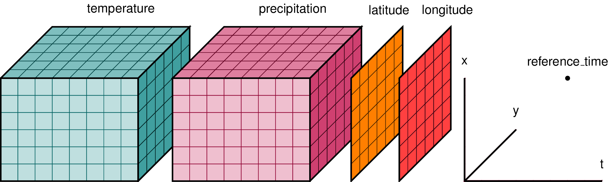
grid_mapping: spatial_refStructure de l’ensemble de données Xarray
Un « Dataset » peut être considéré comme une structure de dictionnaire regroupant les données, les dimensions et les attributs. Les variables d’un objet « Dataset » sont appelées « DataArrays » et elles partagent des dimensions avec l’objet « Dataset » de niveau supérieur. La figure ci-dessous fournit un exemple illustratif :
Pour accéder à une variable, nous pouvons y accéder comme s’il s’agissait d’un dictionnaire Python, ou en utilisant la notation « . », ce qui est plus pratique.
[5]:
ds["green"]
#or alternatively
ds.green
[5]:
<xarray.DataArray 'green' (time: 12, y: 601, x: 483)>
[3483396 values with dtype=uint16]
Coordinates:
* time (time) datetime64[ns] 2018-01-03T08:31:05 ... 2018-02-27T08:...
* y (y) float64 -2.519e+06 -2.519e+06 ... -2.507e+06 -2.507e+06
* x (x) float64 2.378e+06 2.378e+06 ... 2.388e+06 2.388e+06
spatial_ref int32 ...
Attributes:
units: 1
nodata: 0
crs: EPSG:6933
grid_mapping: spatial_refLes dimensions sont également stockées sous forme de tableaux numériques auxquels nous pouvons facilement accéder
[6]:
ds['time']
#or alternatively
ds.time
[6]:
<xarray.DataArray 'time' (time: 12)>
array(['2018-01-03T08:31:05.000000000', '2018-01-08T08:34:01.000000000',
       '2018-01-13T08:30:41.000000000', '2018-01-18T08:30:42.000000000',
       '2018-01-23T08:33:58.000000000', '2018-01-28T08:30:20.000000000',
       '2018-02-07T08:30:53.000000000', '2018-02-12T08:31:43.000000000',
       '2018-02-17T08:23:09.000000000', '2018-02-17T08:35:40.000000000',
       '2018-02-22T08:34:52.000000000', '2018-02-27T08:31:36.000000000'],
      dtype='datetime64[ns]')
Coordinates:
* time (time) datetime64[ns] 2018-01-03T08:31:05 ... 2018-02-27T08:...
spatial_ref int32 ...Les métadonnées sont appelées attributs et sont stockées en interne sous « .attrs », mais la même notation pratique « . » s’applique à elles.
[7]:
ds.attrs['crs']

#or alternatively

ds.crs
[7]:
'EPSG:6933'
Les DataArrays stockent leurs données en interne sous forme de tableaux numpy multidimensionnels. Mais ces tableaux contiennent des dimensions ou des étiquettes qui facilitent la gestion des données. Pour accéder au tableau numpy sous-jacent d’un « DataArray », nous pouvons utiliser la notation « .values ».
[8]:
arr = ds.green.values

type(arr), arr.shape
[8]:
(numpy.ndarray, (12, 601, 483))
Indexage
Xarray propose deux méthodes différentes pour sélectionner des données. Cela inclut l’approche « isel() », où les données peuvent être sélectionnées en fonction de leur index (comme numpy).
[9]:
print(ds.time.values)

ss = ds.green.isel(time=0)
ss
['2018-01-03T08:31:05.000000000' '2018-01-08T08:34:01.000000000'
 '2018-01-13T08:30:41.000000000' '2018-01-18T08:30:42.000000000'
 '2018-01-23T08:33:58.000000000' '2018-01-28T08:30:20.000000000'
 '2018-02-07T08:30:53.000000000' '2018-02-12T08:31:43.000000000'
 '2018-02-17T08:23:09.000000000' '2018-02-17T08:35:40.000000000'
 '2018-02-22T08:34:52.000000000' '2018-02-27T08:31:36.000000000']
[9]:
<xarray.DataArray 'green' (y: 601, x: 483)>
array([[1214, 1232, 1406, ..., 3436, 4252, 4300],
       [1214, 1334, 1378, ..., 2006, 2602, 4184],
       [1274, 1340, 1554, ..., 2436, 1858, 1890],
       ...,
       [1142, 1086, 1202, ..., 1096, 1074, 1092],
       [1188, 1258, 1190, ..., 1058, 1138, 1138],
       [1152, 1134, 1074, ..., 1086, 1116, 1100]], dtype=uint16)
Coordinates:
    time         datetime64[ns] 2018-01-03T08:31:05
  * y            (y) float64 -2.519e+06 -2.519e+06 ... -2.507e+06 -2.507e+06
  * x            (x) float64 2.378e+06 2.378e+06 ... 2.388e+06 2.388e+06
    spatial_ref  int32 ...
Attributes:
    units:         1
    nodata:        0
    crs:           EPSG:6933
grid_mapping: spatial_refOu l’approche « sel() », utilisée pour sélectionner des données en fonction de leur dimension de valeur d’étiquette.
[10]:
ss = ds.green.sel(time='2018-01-08')
ss
[10]:
<xarray.DataArray 'green' (time: 1, y: 601, x: 483)>
array([[[1270, 1280, ..., 4228, 3950],
        [1266, 1332, ..., 3880, 4372],
        ...,
        [1172, 1180, ..., 1154, 1190],
        [1242, 1204, ..., 1192, 1170]]], dtype=uint16)
Coordinates:
  * time         (time) datetime64[ns] 2018-01-08T08:34:01
  * y            (y) float64 -2.519e+06 -2.519e+06 ... -2.507e+06 -2.507e+06
  * x            (x) float64 2.378e+06 2.378e+06 ... 2.388e+06 2.388e+06
    spatial_ref  int32 ...
Attributes:
    units:         1
    nodata:        0
    crs:           EPSG:6933
grid_mapping: spatial_refLe découpage des données est également utilisé pour sélectionner un sous-ensemble de données.
[11]:
ss.x.values[100]
[11]:
2380390.0
[12]:
ss = ds.green.sel(time='2018-01-08', x=slice(2378390,2380390))
ss
[12]:
<xarray.DataArray 'green' (time: 1, y: 601, x: 101)>
array([[[1270, 1280, ..., 1416, 1290],
        [1266, 1332, ..., 1368, 1274],
        ...,
        [1172, 1180, ..., 1086,  991],
        [1242, 1204, ..., 1019,  986]]], dtype=uint16)
Coordinates:
  * time         (time) datetime64[ns] 2018-01-08T08:34:01
  * y            (y) float64 -2.519e+06 -2.519e+06 ... -2.507e+06 -2.507e+06
  * x            (x) float64 2.378e+06 2.378e+06 2.378e+06 ... 2.38e+06 2.38e+06
    spatial_ref  int32 ...
Attributes:
    units:         1
    nodata:        0
    crs:           EPSG:6933
grid_mapping: spatial_refXarray propose de nombreuses fonctions pour transformer et analyser facilement les « Datasets » et les « DataArrays ». Par exemple, pour calculer la moyenne spatiale, l’écart type ou la somme de la bande verte :
[13]:
print("Mean of green band:", ds.green.mean().values)
print("Standard deviation of green band:", ds.green.std().values)
print("Sum of green band:", ds.green.sum().values)
Mean of green band: 4141.488778766468
Standard deviation of green band: 3775.5536474649584
Sum of green band: 14426445446
Traçage de données avec Matplotlib
Le traçage est également intégré de manière pratique dans la bibliothèque.
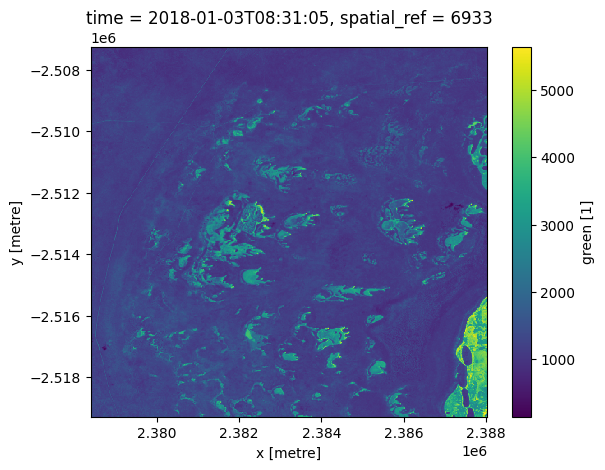
[14]:
ds["green"].isel(time=0).plot()
[14]:
<matplotlib.collections.QuadMesh at 0x7f88d342bd30>
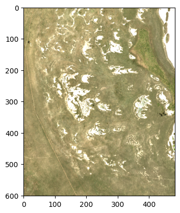
mais nous pouvons toujours faire les choses manuellement en utilisant numpy et matplotlib si vous le souhaitez :
[15]:
rgb = np.dstack((ds.red.isel(time=0).values, ds.green.isel(time=0).values, ds.blue.isel(time=0).values))
rgb = np.clip(rgb, 0, 2000) / 2000

plt.imshow(rgb);
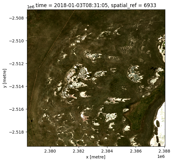
Mais comparez ce qui précède à l’enchaînement élégant d’opérations dans xarray :
[16]:
ds[['red', 'green', 'blue']].isel(time=0).to_array().plot.imshow(robust=True, figsize=(6, 6));
Étapes suivantes recommandées
Pour des informations plus avancées sur l’utilisation de Jupyter Notebooks ou JupyterLab, vous pouvez explorer la page de documentation de JupyterLab.
Pour continuer à travailler sur les cahiers de ce guide du débutant, les cahiers suivants sont conçus pour être travaillés dans l’ordre suivant :
Introduction à xarray (ce notebook)
Une fois que vous avez terminé les huit didacticiels ci-dessus, rejoignez les utilisateurs avancés pour explorer :
Le répertoire « Datasets » du référentiel, où vous pouvez explorer en profondeur les produits DE Africa.
Le répertoire « Code fréquemment utilisé », qui contient un livre de recettes de techniques et méthodes courantes pour l’analyse des données DE Africa.
Le répertoire « Exemples du monde réel », qui fournit des flux de travail plus complexes et des études de cas d’analyse.
Informations Complémentaires
Licence : Le code de ce carnet est sous licence Apache, version 2.0 <https://www.apache.org/licenses/LICENSE-2.0>. Les données de Digital Earth Africa sont sous licence Creative Commons par attribution 4.0 <https://creativecommons.org/licenses/by/4.0/>.
Contact : Si vous avez besoin d’aide, veuillez poster une question sur le canal Slack Open Data Cube <http://slack.opendatacube.org/>`__ ou sur le GIS Stack Exchange en utilisant la balise open-data-cube (vous pouvez consulter les questions posées précédemment ici). Si vous souhaitez signaler un problème avec ce bloc-notes, vous pouvez en déposer un sur Github.
Dernier test :
[17]:
from datetime import datetime
datetime.today().strftime('%Y-%m-%d')
[17]:
'2023-08-11'