Introduction à Numpy
Prérequis : Les utilisateurs de ce notebook doivent avoir une compréhension de base de :
Comment exécuter un Jupyter notebook
Mots-clés guide du débutant; numpy, package python; numpy, package python; matplotlib
Aperçu
Numpy est une bibliothèque Python qui ajoute la prise en charge de grands tableaux multidimensionnels et de mesures, ainsi qu’une grande collection de fonctions mathématiques de haut niveau pour opérer sur ces tableaux. Vous trouverez plus d’informations sur les tableaux Numpy ici <https://en.wikipedia.org/wiki/NumPy>.
Description
Ce bloc-notes est conçu pour présenter aux utilisateurs les tableaux Numpy en utilisant du code Python dans les blocs-notes Jupyter via JupyterLab.
Les sujets abordés comprennent :
Comment utiliser les fonctions Numpy dans une cellule Jupyter Notebook
Utilisation de l’indexation pour explorer les données d’un tableau Numpy multidimensionnel
Types de données Numpy, diffusion et booléens
Utiliser Matplotlib pour tracer des données Numpy
Commencer
Pour exécuter ce bloc-notes, exécutez toutes les cellules du bloc-notes en commençant par la cellule « Charger les packages ». Pour obtenir de l’aide sur l’exécution des cellules du bloc-notes, reportez-vous au bloc-notes Jupyter Notebooks <01_Jupyter_notebooks.ipynb>`__.
Charger des paquets
Pour pouvoir utiliser numpy, nous devons importer la bibliothèque en utilisant le mot spécial « import ». De plus, pour éviter de taper « numpy » à chaque fois que nous voulons utiliser l’une de ses fonctions, nous pouvons fournir un alias en utilisant le mot spécial « as » :
[1]:
import numpy as np
Introduction à Numpy
Maintenant, nous avons accès à toutes les fonctions disponibles dans « numpy » en tapant « np.name_of_function ». Par exemple, l’équivalent de « 1 + 1 » en Python peut être fait dans « numpy » :
[2]:
np.add(1,1)
[2]:
2
Même si cela peut ne pas sembler très utile au premier abord, même des opérations simples comme celle-ci peuvent être beaucoup plus rapides dans « numpy » que dans Python standard lors de l’utilisation de nombreux nombres (grands tableaux).
Pour accéder à la documentation expliquant comment une fonction est utilisée, ses paramètres d’entrée et son format de sortie, nous pouvons appuyer sur « Maj+Tab » après le nom de la fonction. Essayez ceci dans la cellule ci-dessous
[3]:
np.add
[3]:
<ufunc 'add'>
Par défaut, le résultat d’une fonction ou d’une opération est affiché sous la cellule contenant le code. Si nous souhaitons réutiliser ce résultat pour une opération ultérieure, nous pouvons l’affecter à une variable :
[4]:
a = np.add(2,3)
Le contenu de cette variable peut être affiché à tout moment en tapant le nom de la variable dans une nouvelle cellule :
[5]:
a
[5]:
5
Tableaux Numpy
Le concept de base de numpy est le « tableau », qui est équivalent à des listes de nombres mais peut être multidimensionnel. Pour déclarer un tableau numpy, nous faisons :
[6]:
np.array([1,2,3,4,5,6,7,8,9])
[6]:
array([1, 2, 3, 4, 5, 6, 7, 8, 9])
La plupart des fonctions et opérations définies dans numpy peuvent être appliquées aux tableaux. Par exemple, avec l’opération précédente :
[7]:
arr1 = np.array([1,2,3,4])
arr2 = np.array([3,4,5,6])

np.add(arr1, arr2)
[7]:
array([ 4, 6, 8, 10])
Mais une notation plus simple et plus pratique peut également être utilisée :
[8]:
arr1 + arr2
[8]:
array([ 4, 6, 8, 10])
Indexage
Les tableaux peuvent être découpés en tranches et en dés. Nous pouvons obtenir des sous-ensembles de tableaux en utilisant la notation d’indexation qui est « [start:end:stride] ». Voyons ce que cela signifie :
[9]:
arr = np.array([0,1,2,3,4,5,6,7,8,9,10,11,12,13,14,15])

print('6th element in the array:', arr[5])
print('6th element to the end of array', arr[5:])
print('start of array to the 5th element', arr[:5])
print('every second element', arr[::2])
6th element in the array: 5
6th element to the end of array [ 5  6  7  8  9 10 11 12 13 14 15]
start of array to the 5th element [0 1 2 3 4]
every second element [ 0  2  4  6  8 10 12 14]
Essayez d’expérimenter avec les indices pour comprendre la signification de « start », « end » et « stride ». Que se passe-t-il si vous ne spécifiez pas de début ? Quelle valeur numpy utilise-t-il à la place ? Notez que les index numpy commencent à « 0 », la même convention utilisée dans les listes Python.
Les index peuvent également être négatifs, ce qui signifie que vous commencez à compter à partir de la fin. Par exemple, pour sélectionner les 2 derniers éléments d’un tableau, nous pouvons faire :
[10]:
arr[-2:]
[10]:
array([14, 15])
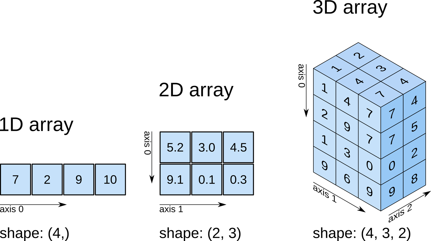
Tableaux multidimensionnels
Les tableaux Numpy peuvent avoir plusieurs dimensions. Par exemple, nous définissons un tableau (1,9) à 2 dimensions en utilisant des crochets imbriqués :
[11]:
np.array([[1,2,3,4,5,6,7,8,9]])
[11]:
array([[1, 2, 3, 4, 5, 6, 7, 8, 9]])
Pour visualiser la forme ou les dimensions d’un tableau numpy, nous pouvons ajouter le suffixe « .shape »
[12]:
print(np.array([1,2,3,4,5,6,7,8,9]).shape)
print(np.array([[1,2,3,4,5,6,7,8,9]]).shape)
print(np.array([[1],[2],[3],[4],[5],[6],[7],[8],[9]]).shape)
(9,)
(1, 9)
(9, 1)
Tout tableau peut être remodelé en différentes formes à l’aide de la fonction « reshape » :
[13]:
np.array([1,2,3,4,5,6,7,8]).reshape((2,4))
[13]:
array([[1, 2, 3, 4],
       [5, 6, 7, 8]])
Si vous craignez de devoir saisir autant de crochets, il existe des moyens plus simples et plus pratiques de procéder de la même manière :
[14]:
print(np.array([1,2,3,4,5,6,7,8,9]).reshape(1,9).shape)
print(np.array([1,2,3,4,5,6,7,8,9]).reshape(9,1).shape)
print(np.array([1,2,3,4,5,6,7,8,9]).reshape(3,3).shape)
(1, 9)
(9, 1)
(3, 3)
Il existe également des raccourcis pour déclarer des tableaux communs sans avoir à saisir tous leurs éléments :
[15]:
print(np.arange(9))
print(np.ones((3,3)))
print(np.zeros((2,2,2)))
[0 1 2 3 4 5 6 7 8]
[[1. 1. 1.]
 [1. 1. 1.]
 [1. 1. 1.]]
[[[0. 0.]
  [0. 0.]]

 [[0. 0.]
  [0. 0.]]]
Opérations arithmétiques
Numpy possède de nombreuses fonctions arithmétiques utiles. Ci-dessous, nous en présentons quelques-unes, telles que la moyenne, l’écart type et la somme des éléments d’un tableau. Ces opérations peuvent être effectuées soit sur l’ensemble du tableau, soit sur une dimension spécifiée.
[16]:
arr = np.arange(9).reshape((3,3))
print(arr)
[[0 1 2]
 [3 4 5]
 [6 7 8]]
[17]:
print('Mean of all elements in the array:', np.mean(arr))
print('Std dev of all elements in the array:', np.std(arr))
print('Sum of all elements in the array:', np.sum(arr))
Mean of all elements in the array: 4.0
Std dev of all elements in the array: 2.581988897471611
Sum of all elements in the array: 36
[18]:
print('Mean of elements in array axis 0:', np.mean(arr, axis=0))
print('Mean of elements in array axis 1:', np.mean(arr, axis=1))
Mean of elements in array axis 0: [3. 4. 5.]
Mean of elements in array axis 1: [1. 4. 7.]
Types de données Numpy
Les tableaux Numpy peuvent contenir des valeurs numériques de différents types. Ces types peuvent être divisés en ces groupes :
Entiers
Non signé
8 bits : « uint8 »
16 bits : « uint16 »
32 bits : « uint32 »
64 bits : « uint64 »
Signé
8 bits : « int8 »
16 bits : « int16 »
32 bits : « int32 »
64 bits : « int64 »
Flotteurs
32 bits : « float32 »
64 bits : « float64 »
Nous pouvons spécifier le type d’un tableau lorsque nous le déclarons, ou modifier le type de données d’un tableau existant avec les expressions suivantes :
[19]:
#set datatype dwhen declaring array
arr = np.arange(5, dtype=np.uint8)
print('Integer datatype:', arr)

arr = arr.astype(np.float32)
print('Float datatype:', arr)
Integer datatype: [0 1 2 3 4]
Float datatype: [0. 1. 2. 3. 4.]
Radiodiffusion
Le terme « diffusion » décrit la manière dont numpy traite les tableaux de formes différentes lors des opérations arithmétiques. Sous réserve de certaines contraintes, le tableau le plus petit est « diffusé » sur le tableau le plus grand afin qu’ils aient des formes compatibles. La diffusion fournit un moyen de vectoriser les opérations sur les tableaux afin que la boucle se produise en C au lieu de Python. Cela peut rendre les opérations très rapides.
[20]:
a = np.zeros((3,3))
print(a)

a = a + 1

print(a)
[[0. 0. 0.]
 [0. 0. 0.]
 [0. 0. 0.]]
[[1. 1. 1.]
 [1. 1. 1.]
 [1. 1. 1.]]
[21]:
a = np.arange(9).reshape((3,3))

b = np.arange(3)

a + b
[21]:
array([[ 0,  2,  4],
       [ 3,  5,  7],
       [ 6,  8, 10]])
Booléens
Il existe un type binaire dans numpy appelé boolean qui encode les valeurs « True » et « False ». Par exemple :
[22]:
arr = (arr > 0)

print(arr)

arr.dtype
[False True True True True]
[22]:
dtype('bool')
Les types booléens sont très pratiques pour indexer et sélectionner des parties d’images comme nous le verrons plus tard. De nombreuses fonctions numpy fonctionnent également avec les types booléens.
[23]:
print("Number of 'Trues' in arr:", np.count_nonzero(arr))

#create two boolean arrays
a = np.array([1,1,0,0], dtype=np.bool_)
b = np.array([1,0,0,1], dtype=np.bool_)

#compare where they match
np.logical_and(a, b)
Number of 'Trues' in arr: 4
[23]:
array([ True, False, False, False])
Introduction à Matplotlib
Cette deuxième partie présente matplotlib, une bibliothèque Python permettant de tracer des tableaux numpy sous forme d’images. Pour les besoins de ce tutoriel, nous allons utiliser une partie de matplotlib appelée pyplot. Nous l’importons en faisant :
[24]:
%matplotlib inline

import numpy as np
from matplotlib import pyplot as plt
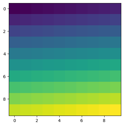
Une image peut être vue comme un tableau à 2 dimensions. Pour visualiser le contenu d’un tableau numpy :
[25]:
arr = np.arange(100).reshape(10,10)

print(arr)

plt.imshow(arr)
[[ 0  1  2  3  4  5  6  7  8  9]
 [10 11 12 13 14 15 16 17 18 19]
 [20 21 22 23 24 25 26 27 28 29]
 [30 31 32 33 34 35 36 37 38 39]
 [40 41 42 43 44 45 46 47 48 49]
 [50 51 52 53 54 55 56 57 58 59]
 [60 61 62 63 64 65 66 67 68 69]
 [70 71 72 73 74 75 76 77 78 79]
 [80 81 82 83 84 85 86 87 88 89]
 [90 91 92 93 94 95 96 97 98 99]]
[25]:
<matplotlib.image.AxesImage at 0x7fa9df19d660>
Nous pouvons utiliser la bibliothèque Pyplot pour charger une image en utilisant la fonction « imread » :
[26]:
im = np.copy(plt.imread('../Supplementary_data/06_Intro_to_numpy/africa.png'))
Affichons cette image en utilisant la fonction « imshow ».
[27]:
plt.imshow(im)
[27]:
<matplotlib.image.AxesImage at 0x7fa9df07f3a0>
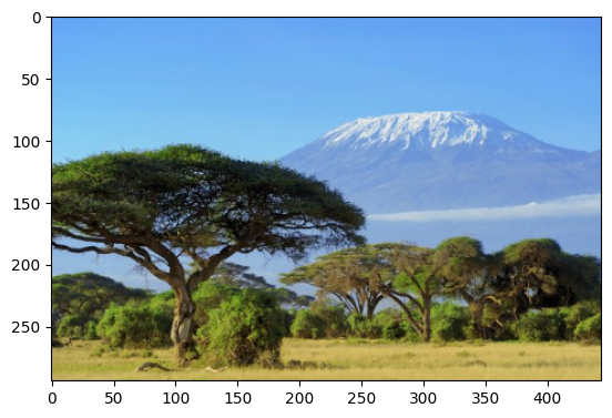
Il s’agit d’une photo libre de droit <https://depositphotos.com/42725091/stock-photo-kilimanjaro.html>__ du mont Kilimandjaro, en Tanzanie. Une image couleur est normalement composée de trois calques contenant les valeurs des pixels rouges, verts et bleus. Lorsque nous affichons une image, nous voyons les trois couleurs combinées.
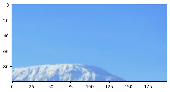
Utilisons la fonctionnalité d’indexation de numpy pour sélectionner une tranche de cette image. Par exemple pour sélectionner le coin supérieur droit :
[28]:
plt.imshow(im[:100,-200:,:])
[28]:
<matplotlib.image.AxesImage at 0x7fa9dcd36860>
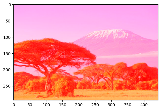
Nous pouvons également remplacer les valeurs de la couche « rouge » par la valeur 255, ce qui rend l’image « rougeâtre ». Essayez :
[29]:
im[:,:,0] = 255
plt.imshow(im)
Clipping input data to the valid range for imshow with RGB data ([0..1] for floats or [0..255] for integers).
[29]:
<matplotlib.image.AxesImage at 0x7fa9dcdc0550>
Étapes suivantes recommandées
Pour des informations plus avancées sur l’utilisation de Jupyter Notebooks ou JupyterLab, vous pouvez explorer la page de documentation de JupyterLab.
Pour continuer à travailler sur les cahiers de ce guide du débutant, les cahiers suivants sont conçus pour être travaillés dans l’ordre suivant :
Introduction à numpy (ce notebook)
Une fois que vous avez terminé les huit didacticiels ci-dessus, rejoignez les utilisateurs avancés pour explorer :
Le répertoire « Datasets » du référentiel, où vous pouvez explorer en profondeur les produits DE Africa.
Le répertoire « Code fréquemment utilisé », qui contient un livre de recettes de techniques et méthodes courantes pour l’analyse des données DE Africa.
Le répertoire « Exemples du monde réel », qui fournit des flux de travail plus complexes et des études de cas d’analyse.
Informations Complémentaires
Licence : Le code de ce carnet est sous licence Apache, version 2.0 <https://www.apache.org/licenses/LICENSE-2.0>. Les données de Digital Earth Africa sont sous licence Creative Commons par attribution 4.0 <https://creativecommons.org/licenses/by/4.0/>.
Contact : Si vous avez besoin d’aide, veuillez poster une question sur le canal Slack Open Data Cube <http://slack.opendatacube.org/>`__ ou sur le GIS Stack Exchange en utilisant la balise open-data-cube (vous pouvez consulter les questions posées précédemment ici). Si vous souhaitez signaler un problème avec ce bloc-notes, vous pouvez en déposer un sur Github.
Dernier test :
[30]:
from datetime import datetime
datetime.today().strftime('%Y-%m-%d')
[30]:
'2023-08-11'