Mapping long-term changes in the annual water extent of the Okavango Delta

• Products used: wofs_ls_summary_annual,

Keywords: data used; WOfS, water; extent, analysis; time series, visualisation; animation

Description

The notebook demonstrates how to load, visualise, and analyse the WOfS annual summary product to gather insights into the longer-term extent of the Okavango delta.

---

Getting started

To run this analysis, run all the cells in the notebook, starting with the “Load packages” cell.

Load packages

Import Python packages that are used for the analysis.

%matplotlib inline

# Force GeoPandas to use Shapely instead of PyGEOS
# In a future release, GeoPandas will switch to using Shapely by default.
import os
os.environ['USE_PYGEOS'] = '0'

import datacube
import numpy as np
import xarray as xr
import seaborn as sns
import geopandas as gpd
import matplotlib.pyplot as plt
from IPython.display import Image
from matplotlib.colors import ListedColormap
from matplotlib.patches import Patch

from deafrica_tools.bandindices import calculate_indices
from deafrica_tools.plotting import map_shapefile, xr_animation
from deafrica_tools.dask import create_local_dask_cluster
from deafrica_tools.spatial import xr_rasterize

Set up a Dask cluster

Dask can be used to better manage memory use and conduct the analysis in parallel. For an introduction to using Dask with Digital Earth Africa, see the Dask notebook.

Note: We recommend opening the Dask processing window to view the different computations that are being executed; to do this, see the Dask dashboard in DE Africa section of the Dask notebook.

To activate Dask, set up the local computing cluster using the cell below.

create_local_dask_cluster()

Connect to the datacube

Activate the datacube database, which provides functionality for loading and displaying stored Earth observation data.

dc = datacube.Datacube(app='water_extent')

Analysis parameters

The following cell sets the parameters, which define the area of interest and the length of time to conduct the analysis over.

The parameters are:

• vector_file: The path to the shapefile or geojson that will define the analysis area of the study

• start_year and end_year: The date range to analyse (e.g. ('1990', '2020').

# Define the area of interest
vector_file = 'data/okavango_delta_outline.geojson'

# Define the start year and end year
start_year = '1990'
end_year = '2020'

View the vector data of Interest on an interactive map

#read shapefile
gdf = gpd.read_file(vector_file)

# map_shapefile(gdf, attribute='GRID_CODE')

Load WOfS annual summaries

#Create a query object
bbox=list(gdf.total_bounds)
lon_range = (bbox[0], bbox[2])
lat_range = (bbox[1], bbox[3])

query = {
    'x': lon_range,
    'y': lat_range,
    'resolution': (-30, 30),
    'output_crs':'EPSG:6933',
    'time': (start_year, end_year),
    'dask_chunks':dict(x=1000,y=1000)
}

#load wofs
ds = dc.load(product="wofs_ls_summary_annual",
             **query)

print(ds)

<xarray.Dataset>
Dimensions:      (time: 31, y: 7774, x: 6955)
Coordinates:
  * time         (time) datetime64[ns] 1990-07-02T11:59:59.999999 ... 2020-07...
  * y            (y) float64 -2.279e+06 -2.279e+06 ... -2.512e+06 -2.513e+06
  * x            (x) float64 2.097e+06 2.097e+06 ... 2.305e+06 2.305e+06
    spatial_ref  int32 6933
Data variables:
    count_wet    (time, y, x) int16 dask.array<chunksize=(1, 1000, 1000), meta=np.ndarray>
    count_clear  (time, y, x) int16 dask.array<chunksize=(1, 1000, 1000), meta=np.ndarray>
    frequency    (time, y, x) float32 dask.array<chunksize=(1, 1000, 1000), meta=np.ndarray>
Attributes:
    crs:           epsg:6933
    grid_mapping:  spatial_ref

#create mask
mask = xr_rasterize(gdf,ds)

#mask data
ds = ds.where(mask)

Animating time series

In the next cell, we plot the dataset we loaded above as an animation GIF, using the `xr_animation <../Frequently_used_code/Animated_timeseries.ipynb>`__ function. The output_path will be saved in the directory where the script is found and you can change the names to prevent files overwrite.

out_path = 'results/okavango_annual_water_frequency.gif'

xr_animation(ds=ds,
             output_path=out_path,
             interval=400,
             bands=['frequency'],
             show_text='WOfS Annual Summary',
             show_date = '%Y',
             width_pixels=700,
             annotation_kwargs={'fontsize': 15},
             imshow_kwargs={'cmap': sns.color_palette("mako_r", as_cmap=True), 'vmin': 0.0, 'vmax': 0.9},
             colorbar_kwargs={'colors': 'black'},
             show_colorbar=False)

# Plot animated gif
plt.close()
Image(filename=out_path)

Exporting animation to results/okavango_annual_water_frequency.gif

<IPython.core.display.Image object>

Calculate the annual area of water extent

The number of pixels can be used for the area of the waterbody if the pixel area is known. Run the following cell to generate the necessary constants for performing this conversion.

pixel_length = query["resolution"][1]  # in metres
m_per_km = 1000  # conversion from metres to kilometres
area_per_pixel = pixel_length**2 / m_per_km**2

Threshold WOfS annual frequency to classify water/not-water

Calculates the area of pixels classified as water (i.e. if ds.frequency is > 0.1, then the pixel will be considered open water during the year)

water_threshold = 0.1

#threshold
water_extent = (ds.frequency > water_threshold).persist()


#calculate area
ds_valid_water_area = water_extent.sum(dim=['x', 'y']) * area_per_pixel

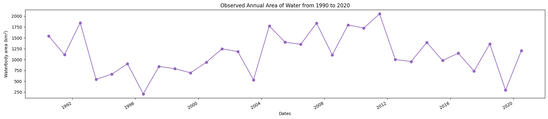
Plot the annual area of open water

plt.figure(figsize=(18, 4))
ds_valid_water_area.plot(marker='o', color='#9467bd')
plt.title(f'Observed Annual Area of Water from {start_year} to {end_year}')
plt.xlabel('Dates')
plt.ylabel('Waterbody area (km$^2$)')
plt.tight_layout()

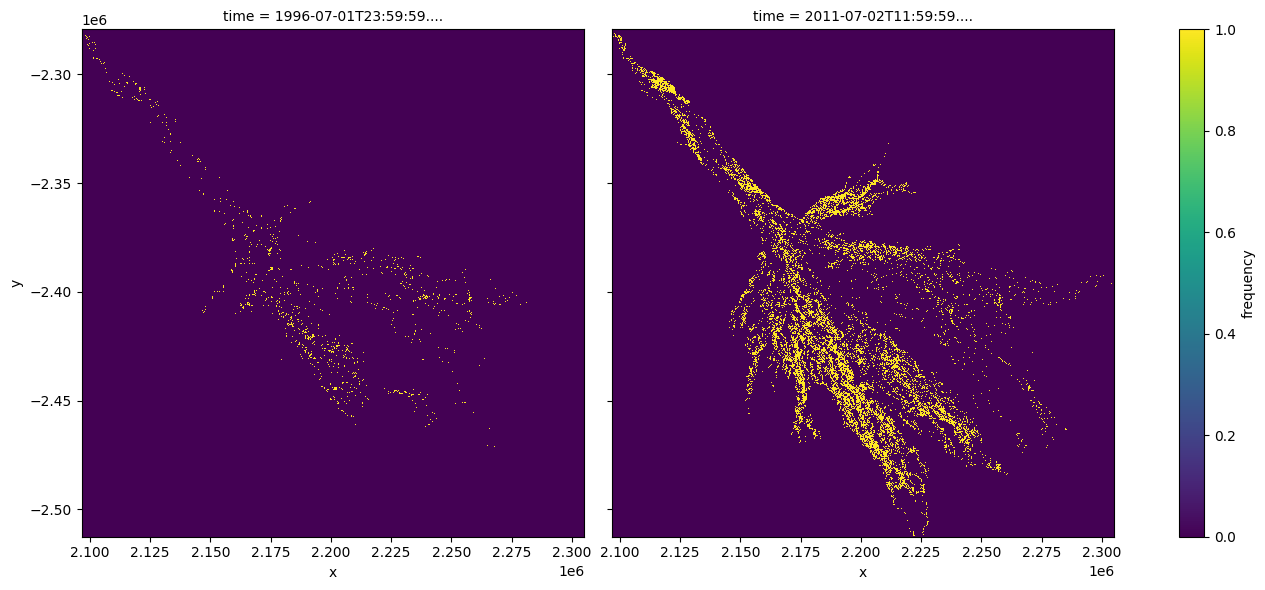
Determine minimum and maximum water extent

The next cell extract the Minimum and Maximum extent of water from the dataset using the min and max functions, we then add the dates to an xarray.DataArray.

min_water_area_date, max_water_area_date =  min(ds_valid_water_area), max(ds_valid_water_area)
time_xr = xr.DataArray([min_water_area_date.time.values, max_water_area_date.time.values], dims=["time"])

print(time_xr)

<xarray.DataArray (time: 2)>
array(['1996-07-01T23:59:59.999999000', '2011-07-02T11:59:59.999999000'],
      dtype='datetime64[ns]')
Dimensions without coordinates: time

Plot the dates when the min and max water extent occur

Plot water classified pixel for the two dates where we have the minimum and maximum surface water extent.

water_extent.sel(time=time_xr).plot.imshow(col="time", col_wrap=2, figsize=(14, 6));

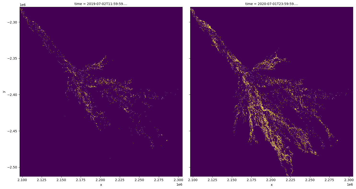
Compare two time periods

The following cells determine the maximum extent of water for two different years. * baseline_year : The baseline year for the analysis * analysis_year : The year to compare to the baseline year

baseline_time = '2019'
analysis_time = '2020'

baseline_ds, analysis_ds = ds_valid_water_area.sel(time=baseline_time), ds_valid_water_area.sel(time=analysis_time)

Plotting

Plot water extent for the two chosen periods.

compare = water_extent.sel(time=[baseline_ds.time.values[0], analysis_ds.time.values[0]])

compare.plot.imshow(col="time",col_wrap=2,figsize=(15, 8), cmap='viridis', add_colorbar=False);

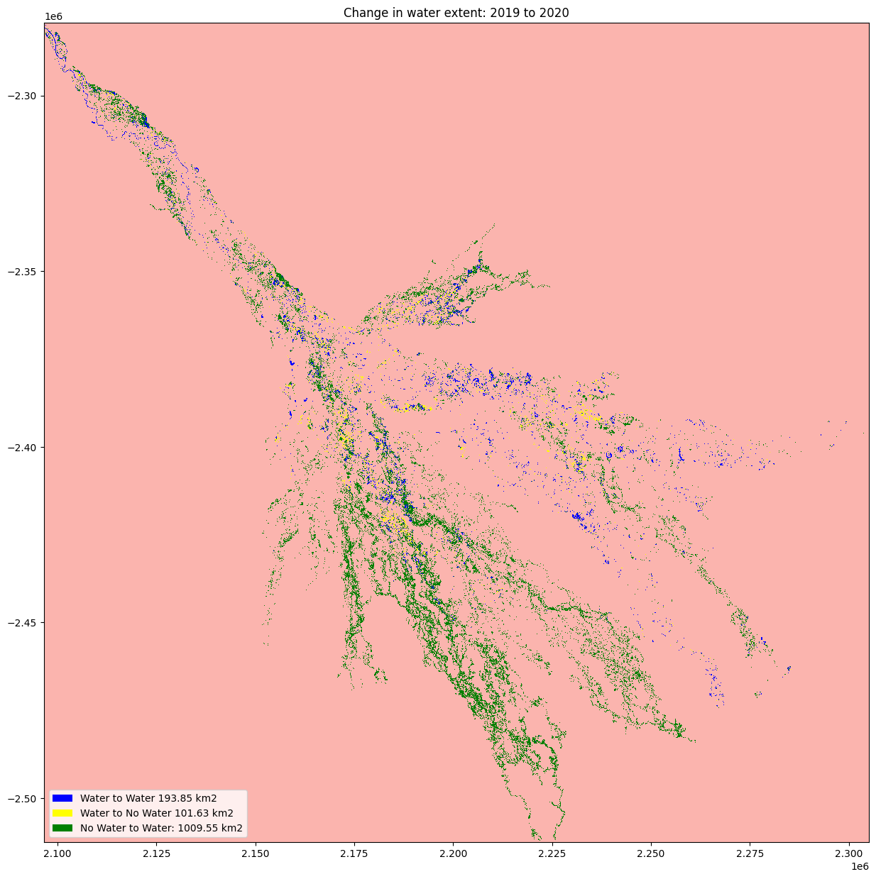
Calculating the change for the two nominated periods

The cells below calculate the amount of water gain, loss and stable for the two periods

analyse_total_value = compare.isel(time=1).astype(int)
change = analyse_total_value - compare.isel(time=0).astype(int)

water_appeared = change.where(change == 1)
permanent_water = change.where((change == 0) & (analyse_total_value == 1))
permanent_land = change.where((change == 0) & (analyse_total_value == 0))
water_disappeared = change.where(change == -1)

The cell below calculate the area of water extent for water_loss, water_gain, permanent water and land

total_area = analyse_total_value.count().values * area_per_pixel
water_apperaed_area = water_appeared.count().values * area_per_pixel
permanent_water_area = permanent_water.count().values * area_per_pixel
water_disappeared_area = water_disappeared.count().values * area_per_pixel

Plotting

The water variables are plotted to visualised the result

water_appeared_color = "Green"
water_disappeared_color = "Yellow"
stable_color = "Blue"
land_color = "Brown"

fig, ax = plt.subplots(1, 1, figsize=(15, 15))

compare[1].plot.imshow(cmap="Pastel1",
                                       add_colorbar=False,
                                       add_labels=False,
                                       ax=ax)
water_appeared.plot.imshow(
    cmap=ListedColormap([water_appeared_color]),
    add_colorbar=False,
    add_labels=False,
    ax=ax,
)
water_disappeared.plot.imshow(
    cmap=ListedColormap([water_disappeared_color]),
    add_colorbar=False,
    add_labels=False,
    ax=ax,
)
permanent_water.plot.imshow(cmap=ListedColormap([stable_color]),
                            add_colorbar=False,
                            add_labels=False,
                            ax=ax)

plt.legend(
    [
        Patch(facecolor=stable_color),
        Patch(facecolor=water_disappeared_color),
        Patch(facecolor=water_appeared_color),
        Patch(facecolor=land_color),
    ],
    [
        f"Water to Water {round(permanent_water_area, 2)} km2",
        f"Water to No Water {round(water_disappeared_area, 2)} km2",
        f"No Water to Water: {round(water_apperaed_area, 2)} km2",
    ],
    loc="lower left",
)

plt.title("Change in water extent: " + baseline_time + " to " + analysis_time);

---

Additional information

License: The code in this notebook is licensed under the Apache License, Version 2.0. Digital Earth Africa data is licensed under the Creative Commons by Attribution 4.0 license.

Contact: If you need assistance, please post a question on the Open Data Cube Slack channel or on the GIS Stack Exchange using the open-data-cube tag (you can view previously asked questions here). If you would like to report an issue with this notebook, you can file one on Github.

Compatible datacube version:

print(datacube.__version__)

1.8.15

Last Tested:

from datetime import datetime
datetime.today().strftime('%Y-%m-%d')

'2023-08-21'