Exporting to Google Drive from the Sandbox

Background

The Google Drive API enables developers to integrate Google Drive functionality into applications, offering access to file storage, sharing, and synchronization capabilities. It allows users to manage files, folders, and permissions programmatically, facilitating seamless integration of cloud storage features into various software solutions. The API supports multiple programming languages and provides robust documentation, making it versatile for a wide range of applications from document management to collaborative platforms. More information can be found here.

PyDrive2 is a wrapper library of google-api-python-client that simplifies many common Google Drive API V2 tasks. The deafrica_tools.externaldrive.authenticate function uses functionality from the PyDrive2 library to authenticate and authorize API requests, enabling seamless integration of Google Drive functionalities directly into data science workflows without user intervention.

To connect to the Google Drive API from the sandbox, follow the instructions here to:

Enable the Google Drive API
Configure the OAuth consent screen
Authorize credentials for a desktop application

At the end of the instructions in step 3, Authorize credentials for a desktop application, you will be asked to save a downloaded JSON file as credentials.json. Once you have completed this step, upload the credentials.json file into the folder /home/jovyan/Supplementary_data/DriveCredentials.

If you wish to use a different folder to store your credentials JSON file and user access token JSON file, once you have uploaded the credentials.json into the desired folder, pass the absolute path of the folder to the variable gdrive_credentials_dir.

⚠️ Security considerations: Users should take care to ensure the security of credentials uploaded into the Sandbox. This includes ensuring they are not incidentally included in uploads to public repositories like GitHub.

Description

This notebook provides a brief introduction to accessing and using Digital Earth Africa’s sandbox with Google Drive:

1 - Authorize and authenticate Google Drive credentials
2 - Interacting with Google Drive using the fsspec filesystem

Getting started

Load packages

Import Python packages that are used for the analysis.

[1]:

import os

import datacube
import matplotlib.pyplot as plt
import odc.algo
import rasterio
import rioxarray
from deafrica_tools.bandindices import calculate_indices
from deafrica_tools.externaldrive import authenticate
from deafrica_tools.plotting import rgb
from odc.geo.xr import write_cog
from pydrive2.fs import GDriveFileSystem

Authorize and authenticate Google Drive credentials

In this section, we will use the authenticate function to handle the authorization and authentication process for Google Drive using PyDrive2. The function ensures the Google Drive API credentials (credentials.json) are correctly loaded, manages the access token (token.json), and returns a GoogleAuth object that we will user to interact with Google Drive (upload, download, or manage files).

Set the folder that the credentials.json file is located in.

[2]:

gdrive_credentials_dir = "/home/jovyan/Supplementary_data/DriveCredentials"

If running the cell below for the first time, a url will be printed in the cell output and you will be prompted to enter a authorization/verification code. To obtain this code perform the following steps:

Copy the url link and open it in your browser.
You will be requested to choose an account. Click on the Google Account that you downloaded the credentials.json JSON file for.
In the next 2 screens click Continue until you come to a page with an Authorization code section.
Copy the code and input it into the input box and press Enter.

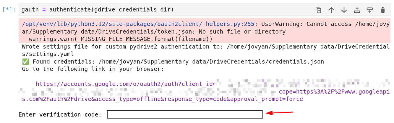
Once you have completed step 5, the cell will run and you will see the message Authentication successful. printed in the cell output.

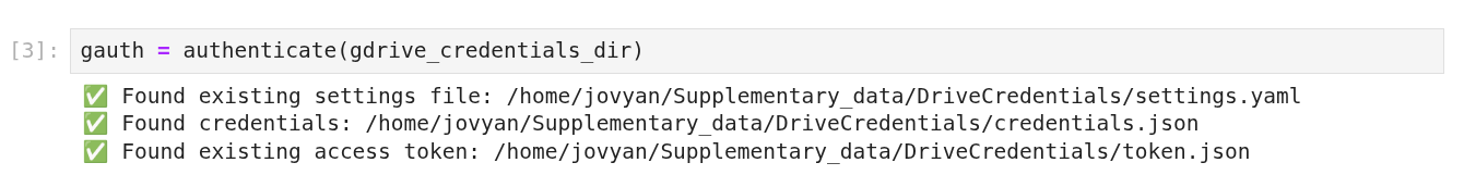
If you have already run the code cell below before and a user access token (token.json) was generated, you will see the following messages printed in the cell output.

authentication

[3]:

gauth =  authenticate(gdrive_credentials_dir)

✅ Found existing settings file: /home/jovyan/Supplementary_data/DriveCredentials/settings.yaml
✅ Found credentials: /home/jovyan/Supplementary_data/DriveCredentials/credentials.json
✅ Found existing access token: /home/jovyan/Supplementary_data/DriveCredentials/token.json

⚠️ You must re-authorize your Google Drive credentials each time you log in (restart your sandbox instance), as the sandbox storage is reset after every session.

Interacting with Google Drive using the fsspec filesystem

PyDrive2 provides an easy way to work with your files through the `fsspec <https://filesystem-spec.readthedocs.io/en/latest/>`__ compatible `GDriveFileSystem <https://docs.iterative.ai/PyDrive2/pydrive2/#pydrive2.fs.GDriveFileSystem>`__. A fsspec filesystem instance offers a large number of methods for getting information about and manipulating files, refer to the fsspec docs on how to use a filesystem.

This section of the notebook will walk you through how to upload, download or manage files using fsspec functionality.

Creating a directory

In this section, we will create a folder in your Google Drive to store outputs from this notebook. All folder and file paths should be absolute and start from the root directory. Paths not starting with root may be considered invalid. root refers to the top-level directory in Google Drive, known as “My Drive”, which serves as the primary heirachy for all user files and folders. This root folder is the starting point for organizing content within Google Drive, and all other folders and files descend from it.

Instantiate a fsspec compatible filesystem instance using GDriveFileSystem and the GoogleAuth object we created in the Authorize and authenticate Google Drive credentials section.

[4]:

# "root" is the root folder of your Google Drive
fs = GDriveFileSystem("root", google_auth = gauth)

Create a folder in your Google Drive.

ℹ️ Info: All folder and file paths should be absolute and start from the root directory. Paths not starting with root may be considered invalid.

[5]:

folder_path = "root/basic_analysis"

[6]:

fs.mkdir(folder_path)

Upload files

In this section we will upload a file on the sandbox into the folder created in the previous section.

Define the absolute path of the file on Google Drive.

[7]:

file_path = "root/basic_analysis/test_gdrive.txt"

Create the text file to be uploaded by writing items in a list to a text file.

[8]:

data_list = [
    "First item to write.",
    "Second item to write.",
    "Third item to write."
]
with open("test_local.txt", 'w') as f:
    for item in data_list:
        f.write(item + '\n')

Upload the file to Google Drive.

[9]:

fs.upload("test_local.txt", file_path)

Verify the file was uploaded by listing items in the folder.

[10]:

fs.ls("root")

[10]:

['root/Colab Notebooks/', 'root/NEMAUseCase/', 'root/basic_analysis/']

[11]:

fs.ls("root/basic_analysis/")

[11]:

['root/basic_analysis/test_gdrive.txt']

Read files

In this section we will read the text file we uploaded to Google Drive in the previous section.

[12]:

file_path = "root/basic_analysis/test_gdrive.txt"

[13]:

# Read files from drive
with fs.open(file_path, "r") as f:
    lines = f.readlines()

# Remove newline characters
lines = [line.strip() for line in lines]

print(lines)

['First item to write.', 'Second item to write.', 'Third item to write.']

Delete files

In this section we will delete the text file we uploaded to Google Drive in the previous section.

[14]:

file_path = "root/basic_analysis/test_gdrive.txt"

[15]:

fs.rm(file_path)

Verify the file was deleted by listing items in the folder.

[16]:

fs.ls("root/basic_analysis/")

[16]:

[]

Writing files

In this section we will write a file directly to Google Drive. This can be a more efficient way to get files onto your Google Drive than having to write them locally first then uploading to Google Drive as seperate steps.

This section will revisit parts of the workflow demonstrated in the Performing a basic analysis notebook notebook.

Define the analysis parameters.

[17]:

# Connect to the datacube
dc = datacube.Datacube(app="Basic_analysis")

# Select a study area and a buffer
# Set the central latitude and longitude
central_lat = -31.5393
central_lon = 18.2682

# Set the buffer to load around the central coordinates
buffer = 0.03

# Compute the bounding box for the study area
study_area_lat = (central_lat - buffer, central_lat + buffer)
study_area_lon = (central_lon - buffer, central_lon + buffer)

Load the Sentinel-2 data for the area of interest.

[18]:

# Set the data source - s2a corresponds to Sentinel-2A
set_product = "s2_l2a"

# Set the date range to load data over
set_time = ("2018-01-01", "2018-01-15")

# Set the measurements/bands to load
# For this analysis, we'll load the red, green, blue and near-infrared bands
set_measurements = [
    "red",
    "blue",
    "green",
    "nir"
]

# Set the coordinate reference system and output resolution
set_crs = 'EPSG:6933'
set_resolution = (-10, 10)

[19]:

dataset = dc.load(
    product=set_product,
    x=study_area_lon,
    y=study_area_lat,
    time=set_time,
    measurements=set_measurements,
    output_crs=set_crs,
    resolution=set_resolution,
    group_by='solar_day'
)
dataset

Select the timestep to use in the workflow.

[20]:

dataset = dataset.isel(time=0)
dataset

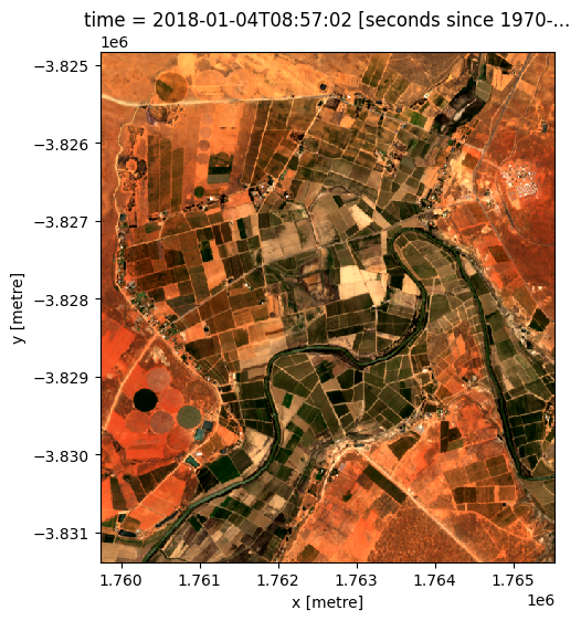
Use the rgb() function to plot the selected time step. The rgb() function maps three data variables/measurements from the loaded dataset to the red, green and blue channels that are used to make a three-colour image.

[21]:

rgb(dataset)

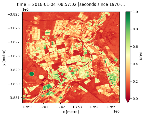
../../../_images/sandbox_notebooks_Frequently_used_code_Integrating_with_Google_Drive_54_0.png

Calculate vegetation health from the selected data.

[22]:

# Convert dataset to float32 datatype so no-data values are set to NaN
dataset =  odc.algo.to_f32(dataset)
# Calcule NDVI
ndvi = calculate_indices(dataset, index="NDVI", satellite_mission="s2", drop=True)
ndvi

Dropping bands ['red', 'blue', 'green', 'nir']

[23]:

# Plot the NDVI band
ndvi["NDVI"].plot(cmap="RdYlGn", vmin=0, vmax=1)
plt.show()

../../../_images/sandbox_notebooks_Frequently_used_code_Integrating_with_Google_Drive_57_0.png

Export the NDVI band to a COG file in your Google drive using the write_cog() command from the odc-geo library and fsspec.

[24]:

cog_file_path = "root/basic_analysis/ndvi.geotiff"

First write the xarray.DataArray into an in memory COG file.

[25]:

da = ndvi.NDVI
da

[26]:

cog_bytes = write_cog(
                    geo_im=ndvi.NDVI,
                    fname=":mem:",
                    overwrite=True,
                )

Write the in-memory file to your Google Drive using fsspec.

[27]:

with fs.open(cog_file_path, "wb") as f:
    f.write(cog_bytes)

Verify the file was uploaded by listing items in the folder.

[28]:

fs.ls("root/basic_analysis/")

[28]:

['root/basic_analysis/ndvi.geotiff']

You can read the GeoTIFF file you’ve uploaded into an xarray.DataArray directly, keeping in mind the constraints highlighted below.

⚠️ Warning: The file object returned by fsspec for Google Drive is streaming-only. It does not supports random access which is required by rasterio in order to read headers, bands, and offsets in a COG. The method demonstrated below will read all bytes into memory. For very large files, this may crash or slow your system.

[29]:

# read all bytes from GDrive
data = fs.open(cog_file_path, "rb").read()
with rasterio.io.MemoryFile(data) as memfile:
    ndvi_from_gdrive = rioxarray.open_rasterio(memfile)

ndvi_from_gdrive

Additional information

License: The code in this notebook is licensed under the Apache License, Version 2.0. Digital Earth Africa data is licensed under the Creative Commons by Attribution 4.0 license.

Contact: If you need assistance, please post a question on the Digital Earth Africa Slack channel or on the GIS Stack Exchange using the open-data-cube tag (you can view previously asked questions here). If you would like to report an issue with this notebook, you can file one on Github.

Compatible datacube version:

[35]:

import datacube
print(datacube.__version__)

1.8.20

Last Tested:

[36]:

from datetime import datetime
datetime.today().strftime('%Y-%m-%d')

[36]:

'2025-12-08'