Phénologie de la végétation dans la réserve de Ruko
Produits utilisés : s2_l2a
Aperçu
La phénologie est l’étude des cycles de vie des plantes et des animaux dans le contexte des saisons. Elle peut être utile pour comprendre les tendances du cycle de vie des cultures et la manière dont les saisons de croissance sont affectées par les changements climatiques. Pour plus d’informations, consultez la page de l’USGS sur la dérivation de la phénologie <https://www.usgs.gov/land-resources/eros/phenology/science/deriving-phenological-metrics-ndvi?qt-science_center_objects=0#qt-science_center_objects>`__.
Description
Ce carnet produira des séries chronologiques annuelles, lissées, unidimensionnelles (moyenne zonale sur une région) d’un indice de végétation par télédétection, tel que le NDVI ou l’EVI. De plus, des statistiques phénologiques de base sont calculées, exportées sur disque sous forme de fichiers csv et annotées sur un tracé.
Plusieurs étapes sont nécessaires pour produire les résultats souhaités :
Charger des données satellite pour une région spécifiée par un fichier vectoriel (shapefile ou geojson)
Mettez en mémoire tampon la couche de masquage des nuages pour mieux masquer les nuages dans les données (le masque de nuages Sentinel-2 est assez médiocre)
Préparez ensuite les données pour l’analyse en supprimant les valeurs erronées (infs), en masquant les eaux de surface et en supprimant les valeurs aberrantes dans l’indice de végétation.
Calculez une moyenne zonale sur la région étudiée (réduisez les dimensions x et y en prenant la moyenne sur tous les pixels pour chaque pas de temps).
Interpolez et lissez les séries chronologiques pour garantir un ensemble de données cohérent avec toutes les lacunes et le bruit supprimés.
Calculez les statistiques phénologiques, signalez les résultats, enregistrez les résultats sur le disque et générez un graphique annoté.
Commencer
Pour exécuter cette analyse, exécutez toutes les cellules du bloc-notes, en commençant par la cellule « Charger les packages ».
Charger des paquets
Chargez les principaux packages Python et les fonctions de support pour l’analyse.
[1]:
%matplotlib inline

import datetime as dt

import datacube
import geopandas as gpd
import matplotlib as mpl
import matplotlib.pyplot as plt
import mpl_toolkits.axisartist as AA
import numpy as np
import pandas as pd
import xarray as xr
from odc.geo.geom import Geometry
from datacube.utils.aws import configure_s3_access
from mpl_toolkits.axes_grid1 import host_subplot

from deafrica_tools.bandindices import calculate_indices
from deafrica_tools.classification import HiddenPrints
from deafrica_tools.dask import create_local_dask_cluster
from deafrica_tools.datahandling import load_ard
from deafrica_tools.plotting import map_shapefile
from deafrica_tools.spatial import xr_rasterize
import deafrica_tools.temporal as ts

configure_s3_access(aws_unsigned=True, cloud_defaults=True)
Configurer un cluster Dask
Dask peut être utilisé pour mieux gérer l’utilisation de la mémoire et effectuer l’analyse en parallèle. Pour une introduction à l’utilisation de Dask avec Digital Earth Africa, consultez le Dask notebook.
Remarque : nous vous recommandons d’ouvrir la fenêtre de traitement Dask pour afficher les différents calculs en cours d’exécution ; pour ce faire, consultez la section Tableau de bord Dask en Afrique de l’Ouest du Dask notebook.
Pour utiliser Dask, configurez le cluster de calcul local à l’aide de la cellule ci-dessous.
[2]:
create_local_dask_cluster(spare_mem='2Gb')
Client
Client-be3a70f2-43c5-11f1-9d4d-ae180e9931c9
| Connection method: Cluster object | Cluster type: distributed.LocalCluster |
| Dashboard: /user/mpho.sadiki@digitalearthafrica.org/proxy/8787/status |
Cluster Info
LocalCluster
a6f87acb
| Dashboard: /user/mpho.sadiki@digitalearthafrica.org/proxy/8787/status | Workers: 1 |
| Total threads: 4 | Total memory: 27.14 GiB |
| Status: running | Using processes: True |
Scheduler Info
Scheduler
Scheduler-c5b2d8b2-65f1-4adb-b2f7-d6edbce2b80d
| Comm: tcp://127.0.0.1:37547 | Workers: 0 |
| Dashboard: /user/mpho.sadiki@digitalearthafrica.org/proxy/8787/status | Total threads: 0 |
| Started: Just now | Total memory: 0 B |
Workers
Worker: 0
| Comm: tcp://127.0.0.1:33581 | Total threads: 4 |
| Dashboard: /user/mpho.sadiki@digitalearthafrica.org/proxy/46879/status | Memory: 27.14 GiB |
| Nanny: tcp://127.0.0.1:34867 | |
| Local directory: /tmp/dask-scratch-space/worker-p4co7pwb | |
Paramètres d’analyse
La cellule suivante définit des paramètres importants pour l’analyse :
« veg_proxy » : indice de bande à utiliser comme proxy pour la santé de la végétation, par exemple « NDVI » ou « EVI »
product: Le produit satellite à charger. Soit Sentinel-2 :'s2_l2a', soit Landsat-8 :'ls8_cl2'shapefile: Le chemin d’accès au fichier vectoriel délimitant la région d’analyse. Peut être un shapefile ou un geojsontime_range: la plage d’années à analyser (par exemple('2017-01-01', '2019-12-30')).« min_gooddata » : la fraction de bonnes données (non troubles) qu’une scène doit avoir avant d’être renvoyée sous forme d’ensemble de données
« résolution » : la résolution en pixels, en mètres, de l’ensemble de données renvoyé
« dask_chunks » : la taille, en nombre de pixels, des morceaux dask sur chaque dimension.
[3]:
veg_proxy = 'NDVI'

product = 's2_l2a'

shapefile='data/Ruko_conservancy.geojson'

time_range = ('2017-01-01', '2020-12-31')

resolution = (-20,20)

dask_chunks = {'x':500, 'y':500}
Se connecter au datacube
Connectez-vous au datacube pour que nous puissions accéder aux données de DE Africa. Le paramètre « app » est un nom unique pour l’analyse qui est basé sur le nom du fichier du notebook.
[4]:
dc = datacube.Datacube(app='Vegetation_phenology')
Voir la région d’intérêt
La cellule suivante affichera la zone sélectionnée sur une carte Web.
[5]:
#First open the shapefile using geopandas
gdf = gpd.read_file(shapefile)
[6]:
map_shapefile(gdf, attribute='ConsrvName')
Charger les données Sentinel-2 masquées par le cloud
La première étape consiste à charger les données Sentinel-2 pour la zone d’intérêt et la plage de temps spécifiées. La fonction « load_ard » est utilisée ici pour charger les données qui ont été masquées pour les filtres de nuages, d’ombre et de qualité, les rendant ainsi prêtes à être analysées.
La cellule directement ci-dessous créera un objet de requête en utilisant la première géométrie du fichier de formes, ainsi que les paramètres que nous avons définis dans la section Paramètres d’analyse ci-dessus.
[7]:
# Create a reusable query
geom = Geometry(geom=gdf.iloc[0].geometry, crs=gdf.crs)

query = {
    "geopolygon": geom,
    'time': time_range,
    'measurements': ['red','nir','green','swir_1'],
    'resolution': resolution,
    'output_crs': 'epsg:6933',
    'group_by':'solar_day'
}
Chargez les données disponibles à partir de S2. Les données de masquage des nuages pour Sentinel-2 sont loin d’être parfaites et les nuages manquants dans les données ont un impact considérable sur les calculs de végétation. load_ard prend en charge les opérations morphologiques sur les bandes de masquage des nuages pour améliorer le masquage des données de mauvaise qualité.
[8]:
filters=[("opening", 3), ("dilation", 2)]

ds = load_ard(
    dc=dc,
    products=['s2_l2a'],
    dask_chunks=dask_chunks,
    mask_filters=filters,
    **query,
)

print(ds)
Using pixel quality parameters for Sentinel 2
Finding datasets
    s2_l2a
Applying morphological filters to pq mask [('opening', 3), ('dilation', 2)]
Applying pixel quality/cloud mask
Returning 267 time steps as a dask array
<xarray.Dataset> Size: 3GB
Dimensions:      (time: 267, y: 1194, x: 607)
Coordinates:
  * time         (time) datetime64[ns] 2kB 2017-01-02T08:07:11 ... 2020-12-27...
  * y            (y) float64 10kB 9.461e+04 9.459e+04 ... 7.077e+04 7.075e+04
  * x            (x) float64 5kB 3.479e+06 3.479e+06 ... 3.491e+06 3.491e+06
    spatial_ref  int32 4B 6933
Data variables:
    red          (time, y, x) float32 774MB dask.array<chunksize=(1, 500, 500), meta=np.ndarray>
    nir          (time, y, x) float32 774MB dask.array<chunksize=(1, 500, 500), meta=np.ndarray>
    green        (time, y, x) float32 774MB dask.array<chunksize=(1, 500, 500), meta=np.ndarray>
    swir_1       (time, y, x) float32 774MB dask.array<chunksize=(1, 500, 500), meta=np.ndarray>
Attributes:
    crs:           EPSG:6933
    grid_mapping:  spatial_ref
/opt/venv/lib/python3.12/site-packages/odc/algo/_masking.py:425: FutureWarning: `binary_opening` is deprecated since version 0.26 and will be removed in version 0.28. Use `skimage.morphology.opening` instead.
  mask = op(mask, _disk(radius, mask.ndim))
/opt/venv/lib/python3.12/site-packages/odc/algo/_masking.py:425: FutureWarning: `binary_dilation` is deprecated since version 0.26 and will be removed in version 0.28. Use `skimage.morphology.dilation` instead. Note the lack of mirroring for non-symmetric footprints (see docstring notes).
  mask = op(mask, _disk(radius, mask.ndim))
/opt/venv/lib/python3.12/site-packages/deafrica_tools/datahandling.py:565: FutureWarning: In a future version of xarray the default value for compat will change from compat='no_conflicts' to compat='override'. This is likely to lead to different results when combining overlapping variables with the same name. To opt in to new defaults and get rid of these warnings now use `set_options(use_new_combine_kwarg_defaults=True) or set compat explicitly.
  ds = xr.merge([ds_data, ds_masks])
Masquer les données satellite avec la forme
[9]:
#create mask
mask = xr_rasterize(gdf,ds)

#mask data
ds = ds.where(mask)

#convert to float 32 to conserve memory
ds=ds.astype(np.float32)
Calculer les indices de végétation et d’eau
[10]:
# Calculate the chosen vegetation proxy index and add it to the loaded data set
ds = calculate_indices(ds, index=[veg_proxy, 'MNDWI'], satellite_mission='s2', drop=True)
Dropping bands ['red', 'nir', 'green', 'swir_1']
Préparer les données pour l’analyse
Supprimez toutes les valeurs NaN ou infinies, masquez l’eau, supprimez toutes les valeurs aberrantes dans l’indice de végétation. Nous réduisons ensuite les données à une série temporelle 1D en calculant la moyenne sur les dimensions x et y.
Nous allons également « calculer » les données sur le cluster dask pour accélérer les calculs ultérieurs. Cette étape prendra 5 à 10 minutes à exécuter puisque nous calculons maintenant tout ce qui précède.
[11]:
# remove any infinite values
ds = ds.where(~np.isinf(ds))
# mask water
ds = ds.where(ds.MNDWI < 0)

#remove outliers (if NDVI greater than 1.0, set to NaN, if less than 0 set to NaN)
ds[veg_proxy] = xr.where(ds[veg_proxy]>1.0, np.nan, ds[veg_proxy])
ds[veg_proxy] = xr.where(ds[veg_proxy]<0, np.nan, ds[veg_proxy])

# create 1D line plots
veg = ds[veg_proxy].mean(['x', 'y']).compute()
/opt/venv/lib/python3.12/site-packages/odc/algo/_masking.py:425: FutureWarning: `binary_opening` is deprecated since version 0.26 and will be removed in version 0.28. Use `skimage.morphology.opening` instead.
  mask = op(mask, _disk(radius, mask.ndim))
/opt/venv/lib/python3.12/site-packages/odc/algo/_masking.py:425: FutureWarning: `binary_dilation` is deprecated since version 0.26 and will be removed in version 0.28. Use `skimage.morphology.dilation` instead. Note the lack of mirroring for non-symmetric footprints (see docstring notes).
  mask = op(mask, _disk(radius, mask.ndim))
/opt/venv/lib/python3.12/site-packages/rasterio/warp.py:385: NotGeoreferencedWarning: Dataset has no geotransform, gcps, or rpcs. The identity matrix will be returned.
  dest = _reproject(
Lisser et interpoler des séries temporelles
En raison de nombreux facteurs (par exemple, des nuages obscurcissant la région, une couverture nuageuse manquante dans la couche SCL), les données seront incomplètes et bruyantes. Ici, nous allons lisser et interpoler les données pour garantir que nous travaillons avec une série chronologique cohérente.
Pour ce faire, nous procédons en deux étapes :
Rééchantillonner les données par pas de temps bimensuels en utilisant la médiane bimensuelle
Calculer une moyenne mobile avec une fenêtre de 4 étapes
[12]:
resample_period='2W'
window=4

veg_smooth = veg.resample(time=resample_period, label='left').median().rolling(time=window, min_periods=1).mean()
# Update the time coordinates of the resampled dataset.
veg_smooth = veg_smooth.assign_coords(time=(veg_smooth.time + np.timedelta64(1, 'W')))
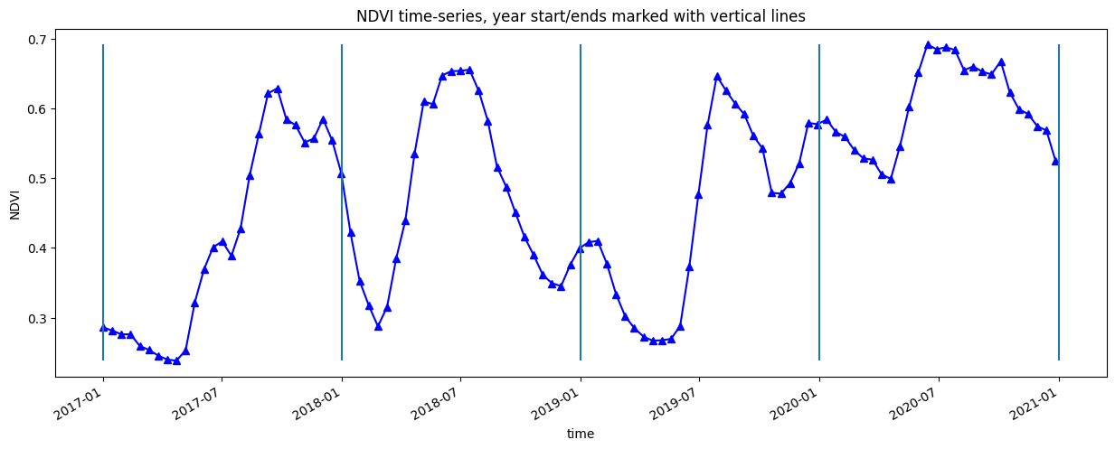
Tracer la série chronologique entière
[13]:
veg_smooth.plot.line('b-^', figsize=(15,5))
_max=veg_smooth.max()
_min=veg_smooth.min()
plt.vlines(np.datetime64('2017-01-01'), ymin=_min, ymax=_max)
plt.vlines(np.datetime64('2018-01-01'), ymin=_min, ymax=_max)
plt.vlines(np.datetime64('2019-01-01'), ymin=_min, ymax=_max)
plt.vlines(np.datetime64('2020-01-01'), ymin=_min, ymax=_max)
plt.vlines(np.datetime64('2021-01-01'), ymin=_min, ymax=_max)
plt.title(veg_proxy+' time-series, year start/ends marked with vertical lines')
plt.ylabel(veg_proxy);
Calculer les statistiques phénologiques de base
Ci-dessous, nous spécifions les statistiques à calculer et la méthode que nous utiliserons pour déterminer les statistiques.
Les acronymes statistiques sont les suivants :
« SOS « – Date de début de saison
» vSOS « - valeur au début de la saison
« POS » - Date de pointe de la saison »
» vPOS « - valeur en haute saison
« EOS « - Date de fin de saison »
« vEOS » - valeur en fin de saison
« Creux » - valeur minimale sur la période de l’ensemble de données
« LOS » - Durée de la saison, mesurée en jours
» AOS « - Amplitude de la saison, la différence entre » vPOS » et « Creux »
» ROG » - Taux de verdissement, taux de changement du début au pic de la saison
« ROS » - Taux de sénescence, taux de changement du pic à la fin de la saison
Les options sont « premier » et « médiane » pour « method_sos », et « dernier » et « médiane » pour « method_eos ».
method_sos : str
        If 'first' then vSOS is estimated as the first positive
        slope on the greening side of the curve. If 'median',
        then vSOS is estimated as the median value of the postive
        slopes on the greening side of the curve.

method_eos : str
        If 'last' then vEOS is estimated as the last negative slope
        on the senescing side of the curve. If 'median', then vEOS is
        estimated as the 'median' value of the negative slopes on the
        senescing side of the curve.
[14]:
basic_pheno_stats = ['SOS','vSOS','POS','vPOS','EOS','vEOS','Trough','LOS','AOS','ROG','ROS']
method_sos = 'first'
method_eos = 'last'
[15]:
# find all the years to assist with plotting
years=veg_smooth.groupby("time.year")

# get list of years in ts to help with looping
years_int = [y[0] for y in years]

# store results in dict
pheno_results = {}

# loop through years and calculate phenology
for year in years_int:
    # select year
    da = dict(years)[year]

    # calculate stats
    stats = ts.xr_phenology(
        da,
        method_sos=method_sos,
        method_eos=method_eos,
        stats=basic_pheno_stats,
        verbose=False,
    )
    # add results to dict
    pheno_results[str(year)] = stats
Imprimez les statistiques phénologiques pour chaque année et écrivez les résultats sur le disque au format .csv
[16]:
df_dict = {}
for key, value in pheno_results.items():
    df_dict_1 = {}
    for b in value.data_vars:
        if value[b].dtype == np.dtype("<M8[ns]") or value[b].dtype == np.dtype("int16"):
            result = pd.to_datetime(value[b].values)
        else:
            result = round(float(value[b].values), 3)
        df_dict_1[b] = result
    df_dict[key] = df_dict_1

df = (pd.DataFrame(df_dict)).T
df.to_csv('results/'+key+'_phenology.csv')
df
[16]:
| SOS | vSOS | POS | vPOS | EOS | vEOS | Trough | LOS | AOS | ROG | ROS | |
|---|---|---|---|---|---|---|---|---|---|---|---|
| 2017 | 2017-04-23 00:00:00 | 0.238 | 2017-09-24 00:00:00 | 0.629 | 2017-12-31 00:00:00 | 0.507 | 0.238 | 252.0 | 0.39 | 0.003 | -0.001 |
| 2018 | 2018-03-11 00:00:00 | 0.315 | 2018-07-15 00:00:00 | 0.655 | 2018-11-18 00:00:00 | 0.349 | 0.287 | 252.0 | 0.368 | 0.003 | -0.002 |
| 2019 | 2019-05-05 00:00:00 | 0.274 | 2019-07-28 00:00:00 | 0.656 | 2019-11-03 00:00:00 | 0.482 | 0.271 | 182.0 | 0.385 | 0.005 | -0.002 |
| 2020 | 2020-04-19 00:00:00 | 0.499 | 2020-07-26 00:00:00 | 0.696 | 2020-12-27 00:00:00 | 0.53 | 0.499 | 252.0 | 0.196 | 0.002 | -0.001 |
Annoter la phénologie sur une parcelle
Cette image sera enregistrée sur le disque dans le dossier « résultats/ »
[17]:
# Figure to which the subplot will be added
fig = plt.figure(figsize=(15, 7))
# Create a subplot that can act as a host to parasitic axes
host = host_subplot(111, figure=fig, axes_class=AA.Axes)
# fig, ax = plt.subplots()


# Function to use to edit the axes of the plot
def adjust_axes(ax):
    # Set the location of the major and minor ticks.
    ax.xaxis.set_major_locator(mpl.dates.MonthLocator())
    ax.xaxis.set_minor_locator(mpl.dates.MonthLocator(bymonthday=16))

    # Format the major and minor tick labels.

    ax.xaxis.set_major_formatter(mpl.ticker.NullFormatter())
    ax.xaxis.set_minor_formatter(mpl.dates.DateFormatter("%b"))


#     # Turn off unnecessary ticks.
    ax.axis["bottom"].minor_ticks.set_visible(False)

    ax.axis["top"].major_ticks.set_visible(False)
    ax.axis["top"].minor_ticks.set_visible(False)

    ax.axis["right"].major_ticks.set_visible(False)
    ax.axis["right"].minor_ticks.set_visible(False)


# find all the years to assist with plotting
years=veg_smooth.groupby('time.year')

# Counter to aid in plotting.
counter = 0

for y, year in years:
    # Grab all the values we need for plotting.
    eos = df.loc[str(y)].EOS
    sos = df.loc[str(y)].SOS
    pos = df.loc[str(y)].POS

    veos = df.loc[str(y)].vEOS
    vsos = df.loc[str(y)].vSOS
    vpos = df.loc[str(y)].vPOS

    if counter == 0:
        ax = host
    else:
        # Create the secondary axis.
        ax = host.twiny()

    # Plot the data
    year.plot(ax=ax, label=y)
    # add start of season

    ax.plot(sos, vsos, "or")
    ax.annotate(
        "SOS",
        xy=(sos, vsos),
        xytext=(-15, 20),
        textcoords="offset points",
        arrowprops=dict(arrowstyle="-|>"),
    )

    # add end of season
    ax.plot(eos, veos, "or")
    ax.annotate(
        "EOS",
        xy=(eos, veos),
        xytext=(0, 20),
        textcoords="offset points",
        arrowprops=dict(arrowstyle="-|>"),
    )

    # add peak of season
    ax.plot(pos, vpos, "or")
    ax.annotate(
        "POS",
        xy=(pos, vpos),
        xytext=(-10, -25),
        textcoords="offset points",
        arrowprops=dict(arrowstyle="-|>"),
    )

    # Set the x-axis limits
    min_x = dt.date(y, 1, 1)
    max_x = dt.date(y, 12, 31)
    ax.set_xlim(min_x, max_x)

    adjust_axes(ax)
    counter += 1


host.legend(labelcolor="linecolor")
host.set_ylim([_min - 0.025, _max.values + 0.05])

plt.ylabel(veg_proxy)
plt.xlabel("Month")

plt.title("Yearly " + veg_proxy);
plt.savefig('results/yearly_phenology_plot.png');
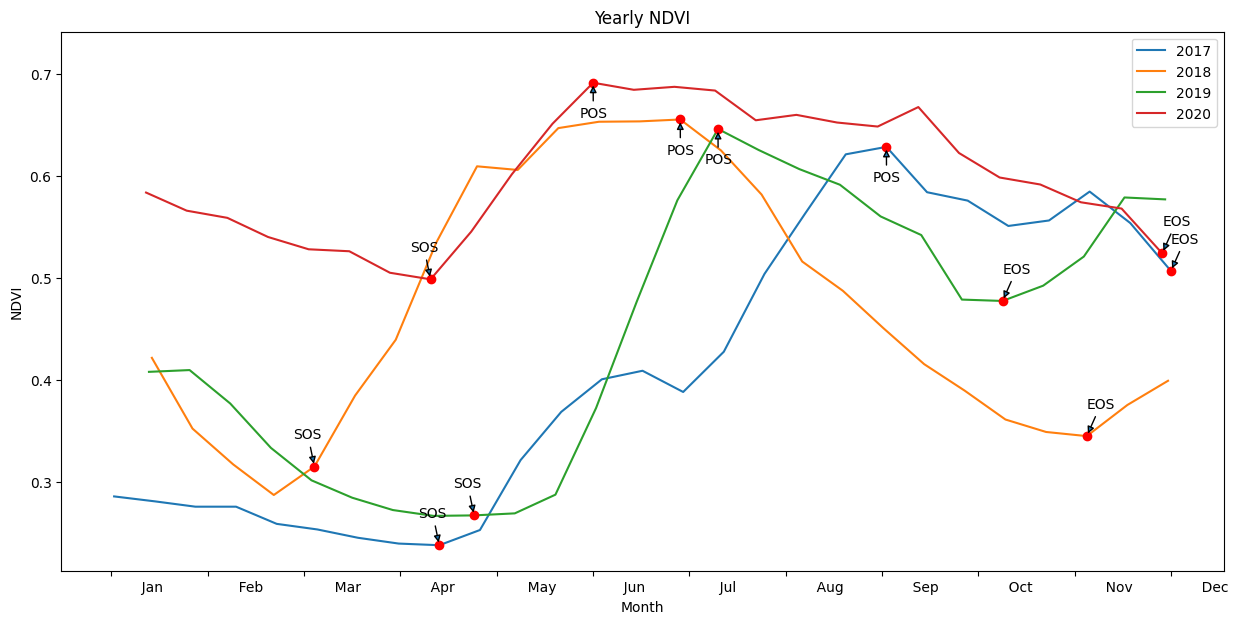
Les statistiques phénologiques de base sont résumées dans un format plus lisible ci-dessous. Nous pouvons comparer les statistiques à un niveau élevé. Des analyses plus approfondies doivent être effectuées à l’aide des exportations .csv dans le dossier /results.
[18]:
print(xr.concat([pheno_results[str(year)] for year in years_int],
                dim=pd.Index(years_int, name='time')).to_dataframe().drop(columns=['spatial_ref']).T.to_string())
time                   2017                 2018                 2019                 2020
SOS     2017-04-23 00:00:00  2018-03-11 00:00:00  2019-05-05 00:00:00  2020-04-19 00:00:00
vSOS               0.238188              0.31534             0.273537              0.49939
POS     2017-09-24 00:00:00  2018-07-15 00:00:00  2019-07-28 00:00:00  2020-07-26 00:00:00
vPOS               0.628646             0.655491             0.655767             0.695777
EOS     2017-12-31 00:00:00  2018-11-18 00:00:00  2019-11-03 00:00:00  2020-12-27 00:00:00
vEOS                0.50702             0.349192             0.481802             0.530077
Trough             0.238188             0.287414             0.271097              0.49939
LOS                   252.0                252.0                182.0                252.0
AOS                0.390459             0.368077              0.38467             0.196387
ROG                0.002535               0.0027              0.00455             0.002004
ROS               -0.001241            -0.002431            -0.001775            -0.001076
Informations Complémentaires
Licence : Le code de ce carnet est sous licence Apache, version 2.0 <https://www.apache.org/licenses/LICENSE-2.0>. Les données de Digital Earth Africa sont sous licence Creative Commons par attribution 4.0 <https://creativecommons.org/licenses/by/4.0/>.
Contact : Si vous avez besoin d’aide, veuillez poster une question sur le canal Slack Open Data Cube <http://slack.opendatacube.org/>`__ ou sur le GIS Stack Exchange en utilisant la balise open-data-cube (vous pouvez consulter les questions posées précédemment ici). Si vous souhaitez signaler un problème avec ce bloc-notes, vous pouvez en déposer un sur Github.
Version de Datacube compatible :
[19]:
print(datacube.__version__)
1.9.13
Dernier test :
[20]:
from datetime import datetime
datetime.today().strftime('%Y-%m-%d')
[20]:
'2026-04-29'