Cahier d’index à couverture verte Mountain (ODD 15.4.2)

Avertissement : Le carnet est en cours de développement. Cet atelier sera un bon forum pour obtenir des commentaires afin d’affiner le carnet. Merci.

Aperçu

Objectif de développement durable 15 :

Protéger, restaurer et promouvoir l’utilisation durable des écosystèmes terrestres, gérer durablement les forêts, lutter contre la désertification, stopper et inverser la dégradation des terres et mettre un terme à la perte de biodiversité.

Objectif 15.4

D’ici à 2030, assurer la conservation des écosystèmes de montagne, y compris leur biodiversité, afin de renforcer leur capacité à fournir des avantages essentiels au développement durable.

Indicateur 15.4.2 : Indice de couverture végétale des montagnes

L’indice de couverture végétale des montagnes (MGCI) est conçu pour mesurer l’étendue et l’évolution de la végétation verte dans les zones de montagne - c’est-à-dire les forêts, les arbustes, les arbres, les pâturages, les terres cultivées, etc. - afin de suivre les progrès vers l’objectif de montagne. Le MGCI est défini comme le pourcentage de couverture végétale sur la surface totale de la région montagneuse d’un pays donné et pour une année de référence donnée. L’objectif de l’indice est de suivre l’évolution de la couverture végétale et d’évaluer ainsi l’état de conservation des écosystèmes de montagne. De plus amples informations sur le MGCI sont disponibles ici <https://www.fao.org/sustainable-development-goals/indicators/1542/en/>`__.

Description

La méthodologie de calcul de l’indice de couverture végétale des montagnes a été initialement développée par la FAO (De Simone et al., 2021).

L’indice de couverture végétale des montagnes est calculé à l’aide de deux couches de descripteurs d’informations :

1. Une couche de description des montagnes : les montagnes peuvent être définies en référence à une variété de paramètres, tels que le climat, l’altitude, l’écologie (Körner et al., 2011) (Karagulle et al., 2017). Cette méthodologie adhère à la définition de la montagne du PNUE-WCMC, s’appuyant à son tour sur la description de la montagne proposée par Kapos et al. (2000).

2. Une couche de description de la végétation : La couche de description de la végétation classe la couverture terrestre en zones vertes et non vertes. La végétation verte comprend à la fois la végétation naturelle et la végétation résultant d’une activité anthropique (par exemple, les cultures, le reboisement, etc.). Les zones non vertes comprennent les zones à végétation très clairsemée, les terres nues, l’eau, la glace/neige permanente et les zones urbaines. La couche de description de la végétation peut être dérivée de différentes manières, mais les cartes de couverture terrestre basées sur la télédétection sont la source de données la plus pratique à cette fin, car elles fournissent les informations requises sur les zones vertes et non vertes d’une manière spatialement explicite et permettent une comparaison dans le temps grâce à l’analyse des changements de couverture terrestre.

Actuellement, la FAO utilise comme solution générale les séries chronologiques de couverture terrestre produites par l’Agence spatiale européenne (ESA) dans le cadre de l’Initiative sur le changement climatique (ICC). De plus amples informations sont disponibles ici <https://hqfao.maps.arcgis.com/home/item.html?id=701f5aea91d141adbc0c4aa0bacb8739>.

Le bloc-notes effectue les opérations suivantes :

1. Calculer la classe de la chaîne de montagnes Kapos pour la zone d’étude

2. Reclasser l’ESA CCI en classification IPCC et verte et non verte

3. Générer l’indice de couverture végétale des montagnes (MGCI)

---

Commencer

Pour exécuter cette analyse, exécutez toutes les cellules du bloc-notes, en commençant par la cellule « Charger les packages ».

Charger des paquets

%matplotlib inline

import os
import datacube
import matplotlib.pyplot as plt
import xarray as xr
import numpy as np
import geopandas as gpd
import pandas as pd
from scipy.ndimage import uniform_filter, maximum_filter, minimum_filter
from odc.geo.xr import write_cog
from odc.geo.geom import Geometry
from odc.geo.crs import CRS

from deafrica_tools.datahandling import load_ard
from deafrica_tools.plotting import rgb, display_map, plot_lulc, map_shapefile
from deafrica_tools.bandindices import calculate_indices
from deafrica_tools.dask import create_local_dask_cluster
from deafrica_tools.spatial import xr_rasterize

from odc.geo.xr import xr_reproject

Configurer un cluster Dask

Dask peut être utilisé pour mieux gérer l’utilisation de la mémoire et effectuer l’analyse en parallèle. Pour une introduction à l’utilisation de Dask avec Digital Earth Africa, consultez le Dask notebook.

Remarque : nous vous recommandons d’ouvrir la fenêtre de traitement Dask pour afficher les différents calculs en cours d’exécution ; pour ce faire, consultez la section Tableau de bord Dask en Afrique de l’Ouest du Dask notebook.

Pour utiliser Dask, configurez le cluster de calcul local à l’aide de la cellule ci-dessous.

create_local_dask_cluster()

/opt/venv/lib/python3.12/site-packages/distributed/node.py:188: UserWarning: Port 8787 is already in use.
Perhaps you already have a cluster running?
Hosting the HTTP server on port 42821 instead
  warnings.warn(

Client

Client-68a21276-3754-11f1-94a2-66901f7a1b9b

Connection method: Cluster object	Cluster type: distributed.LocalCluster
Dashboard: /user/mpho.sadiki@digitalearthafrica.org/proxy/42821/status

Launch dashboard in JupyterLab

Cluster Info

LocalCluster

3eab4926

Dashboard: /user/mpho.sadiki@digitalearthafrica.org/proxy/42821/status	Workers: 1
Total threads: 4	Total memory: 26.21 GiB
Status: running	Using processes: True

Scheduler Info

Scheduler

Scheduler-3db78d04-f3ca-42d2-96d9-81370d11b8e6

Comm: tcp://127.0.0.1:35169	Workers: 0
Dashboard: /user/mpho.sadiki@digitalearthafrica.org/proxy/42821/status	Total threads: 0
Started: Just now	Total memory: 0 B

Workers

Worker: 0

Comm: tcp://127.0.0.1:33959	Total threads: 4
Dashboard: /user/mpho.sadiki@digitalearthafrica.org/proxy/43511/status	Memory: 26.21 GiB
Nanny: tcp://127.0.0.1:46565
Local directory: /tmp/dask-scratch-space/worker-6xdok9ax

Paramètres d’analyse

La cellule suivante définit des paramètres importants pour l’analyse :

• « time » : il s’agit de la période de temps qui nous intéresse pour l’analyse.

• output_crs : Le système de référence de coordonnées vers lequel les données chargées doivent être reprojetées.

• dask_chunks : la taille des morceaux dask, dask divise les données en morceaux gérables qui peuvent être facilement stockés en mémoire.

• output_dir : Le répertoire dans lequel stocker les résultats de l’analyse.

time = 2019

output_crs = "EPSG:6933"

dask_chunks = {"time": 1, "x": 3000, "y": 3000}

# Create the output directory to store the results.
output_dir = "results"
os.makedirs(output_dir, exist_ok=True)

Se connecter au datacube

Connectez-vous au datacube pour que nous puissions accéder aux données de DE Africa. Le paramètre « app » est un nom unique pour l’analyse qui est basé sur le nom du fichier du notebook.

dc = datacube.Datacube(app="mgci")

Sélectionnez un pays

Charger le fichier GeoJSON des pays africains. Ce fichier contient des polygones pour les frontières des pays africains.

african_countries  = gpd.read_file("../../Supplementary_data/MGCI/african_countries.geojson")
african_countries.explore()

Make this Notebook Trusted to load map: File -> Trust Notebook

Listez les pays africains dans GeoJSON.

np.unique(african_countries["COUNTRY"])

array(['Algeria', 'Angola', 'Benin', 'Botswana', 'Burkina Faso',
       'Burundi', 'Cameroon', 'Cape Verde', 'Central African Republic',
       'Chad', 'Comoros', 'Congo-Brazzaville', 'Cote d`Ivoire',
       'Democratic Republic of Congo', 'Djibouti', 'Egypt',
       'Equatorial Guinea', 'Eritrea', 'Ethiopia', 'Gabon', 'Gambia',
       'Ghana', 'Guinea', 'Guinea-Bissau', 'Kenya', 'Lesotho', 'Liberia',
       'Libya', 'Madagascar', 'Malawi', 'Mali', 'Mauritania', 'Morocco',
       'Mozambique', 'Namibia', 'Niger', 'Nigeria', 'Rwanda',
       'Sao Tome and Principe', 'Senegal', 'Sierra Leone', 'Somalia',
       'South Africa', 'Sudan', 'Swaziland', 'Tanzania', 'Togo',
       'Tunisia', 'Uganda', 'Western Sahara', 'Zambia', 'Zimbabwe'],
      dtype=object)

Parmi les pays ci-dessus, vous pouvez en choisir un et le saisir dans la variable de pays ci-dessous.

country = "Rwanda"

idx = african_countries[african_countries['COUNTRY'] == country].index[0]
geom = Geometry(geom=african_countries.iloc[idx].geometry, crs=african_countries.crs)

# Set up daatcube query object.
query = {
    "geopolygon": geom,
    "output_crs": output_crs,
    "dask_chunks": dask_chunks,
}

Charger le jeu de données SRTM DEM à une résolution de 1000 m

ds = dc.load(product="dem_srtm",
             resolution=(-1000, 1000),
             measurements="elevation",
             **query)

### Opération de réduction de quartier

# Implmenting the reducers on the dem results
# var ler = dem.reduceNeighborhood({reducer: ee.Reducer.minMax(),
# kernel: ee.Kernel.circle({radius:7000, units:’meter’})});
def reduce_nei(da, size, pre):
    img = da.values
    if pre == "max":
        img = maximum_filter(img, size=size, mode="nearest")
    else:
        img = minimum_filter(img, size=size, mode="nearest")

    return img


ds_max = ds.elevation.groupby("time").apply(reduce_nei, size=7, pre="max")
ds_min = ds.elevation.groupby("time").apply(reduce_nei, size=7, pre="min")

Calcul de la plage d’élévation locale (LER)

ds["ler_range"] = ds_max - ds_min

Charger le jeu de données dérivées de pente SRTM DEM à une résolution de 30 m

ds_slope = dc.load(product="dem_srtm_deriv",
                   resolution=(-30, 30),
                   measurements="slope",
                   **query)

# Mask using the country polygon.
african_countries = african_countries.to_crs(output_crs)
mask = xr_rasterize(african_countries[african_countries['COUNTRY'] == country],  ds_slope)
ds_slope = ds_slope.where(mask)

Suréchantillonnage du jeu de données dem_strm à une résolution de 1 000 m à 30 m

ds = xr_reproject(src=ds, how=ds_slope.odc.geobox, resampling="nearest")

# Mask using the country polygon.
ds = ds.where(mask)

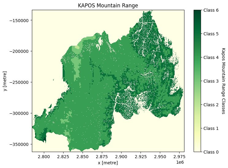
Génération de classes de montagnes de la chaîne de Kapos

classess = [0, 1, 2, 3, 4, 5, 6]
class_label = ["Class 0", "Class 1", "Class 2", "Class 3", "Class 4", "Class 5", "Class 6"]

elevation = ds["elevation"]
slope = ds_slope["slope"]
ler_range = ds["ler_range"]

conditions = [(elevation < 300),
              (elevation > 4500),
              (elevation >= 3500) & (elevation < 4500),
              (elevation >= 2500) & (elevation < 3500),
              (elevation >= 1500) & (elevation < 2500) & (slope > 2),
              (elevation >= 1000) & (elevation < 1500) & ((slope > 5) | (ler_range > 300)),
              (elevation >= 300) & (elevation < 1000) & (ler_range > 300)]

ds["kapo_class"] = xr.DataArray(np.select(conditions, classess),
                                coords={"time": ds.time, "y": ds.y, "x": ds.x},
                                dims=["time", "y", "x"]).astype("int8")

/opt/venv/lib/python3.12/site-packages/distributed/client.py:3387: UserWarning: Sending large graph of size 47.92 MiB.
This may cause some slowdown.
Consider loading the data with Dask directly
 or using futures or delayed objects to embed the data into the graph without repetition.
See also https://docs.dask.org/en/stable/best-practices.html#load-data-with-dask for more information.
  warnings.warn(
/opt/venv/lib/python3.12/site-packages/rasterio/warp.py:385: NotGeoreferencedWarning: Dataset has no geotransform, gcps, or rpcs. The identity matrix will be returned.
  dest = _reproject(
/opt/venv/lib/python3.12/site-packages/distributed/client.py:3387: UserWarning: Sending large graph of size 48.12 MiB.
This may cause some slowdown.
Consider loading the data with Dask directly
 or using futures or delayed objects to embed the data into the graph without repetition.
See also https://docs.dask.org/en/stable/best-practices.html#load-data-with-dask for more information.
  warnings.warn(
/opt/venv/lib/python3.12/site-packages/distributed/client.py:3387: UserWarning: Sending large graph of size 95.87 MiB.
This may cause some slowdown.
Consider loading the data with Dask directly
 or using futures or delayed objects to embed the data into the graph without repetition.
See also https://docs.dask.org/en/stable/best-practices.html#load-data-with-dask for more information.
  warnings.warn(
/opt/venv/lib/python3.12/site-packages/distributed/client.py:3387: UserWarning: Sending large graph of size 95.79 MiB.
This may cause some slowdown.
Consider loading the data with Dask directly
 or using futures or delayed objects to embed the data into the graph without repetition.
See also https://docs.dask.org/en/stable/best-practices.html#load-data-with-dask for more information.
  warnings.warn(

Tracé des classes de la chaîne de montagnes Kapos

kap = ds["kapo_class"].plot(size=6, add_colorbar=False, cmap="YlGn")
kap_c = plt.colorbar(kap)
kap_c.set_ticks(classess)
kap_c.set_ticklabels(class_label)
kap_c.set_label("Kapos Mountain Range Classes", loc="center", labelpad=15, rotation=270)
plt.title("KAPOS Mountain Range")
plt.savefig(f"results/kapos_{country}")
plt.show()

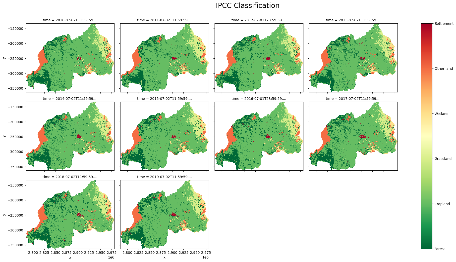
Chargement de l’ensemble de données sur la couverture terrestre de l’Initiative sur les changements climatiques de l’ESA à une résolution de 300 m

# load the data.
ds_cci = dc.load(product="cci_landcover",
                 time=(f'{time-9}', f'{time}'),
                 measurements="classification",
                 resolution=(-300, 300),
                 **query)

# Mask the dataset to the country polygon.
mask = xr_rasterize(african_countries[african_countries['COUNTRY'] == country], ds_cci)
ds_cci = ds_cci.where(mask)

Reclasser la couverture terrestre du CCI selon les classes de couverture terrestre du GIEC

ipcc_classess = ['Forest', 'Cropland', 'Grassland', 'Wetland', 'Other land', 'Settlement']
ipcc_classess_num = [1, 2, 3, 4, 5, 6]

ds_clas = ds_cci['classification']
#IPCC Classification
forest = [50, 60, 61, 62, 70, 71, 72, 80, 81, 82, 90, 100]
cropland = [10, 11, 12, 20, 30, 110]
grassland = [40, 120, 121, 122, 130, 140]
wetland = [160, 170, 180]
otherland = [150, 151, 152, 153, 200, 201, 202, 210, 220]
settlement = [190]

ipcc_condition = [ds_clas.isin(forest),
                  ds_clas.isin(cropland),
                  ds_clas.isin(grassland),
                  ds_clas.isin(wetland),
                  ds_clas.isin(otherland),
                  ds_clas.isin(settlement)]

ds_cci["ipcc_classification"] = xr.DataArray(np.select(ipcc_condition, ipcc_classess_num),
                                             coords={"time": ds_cci.time, "y": ds_cci.y, "x": ds_cci.x},
                                             dims=["time", "y", "x"]).astype("int8").where(mask)

Tracé de la classification du GIEC

clas = ds_cci["ipcc_classification"].plot(col='time',
                                          add_colorbar=False,
                                          figsize = (20, 10),
                                          cmap="RdYlGn_r",
                                          col_wrap = 4)

clas.fig.suptitle("IPCC Classification", ha="center", y=1.05, size=20)
clasp = plt.colorbar(clas._mappables[-1], ax = clas.axs)
clasp.set_ticks(ipcc_classess_num)
clasp.set_ticklabels(ipcc_classess)
plt.savefig(f"results/IPCC_{country}")
plt.show()

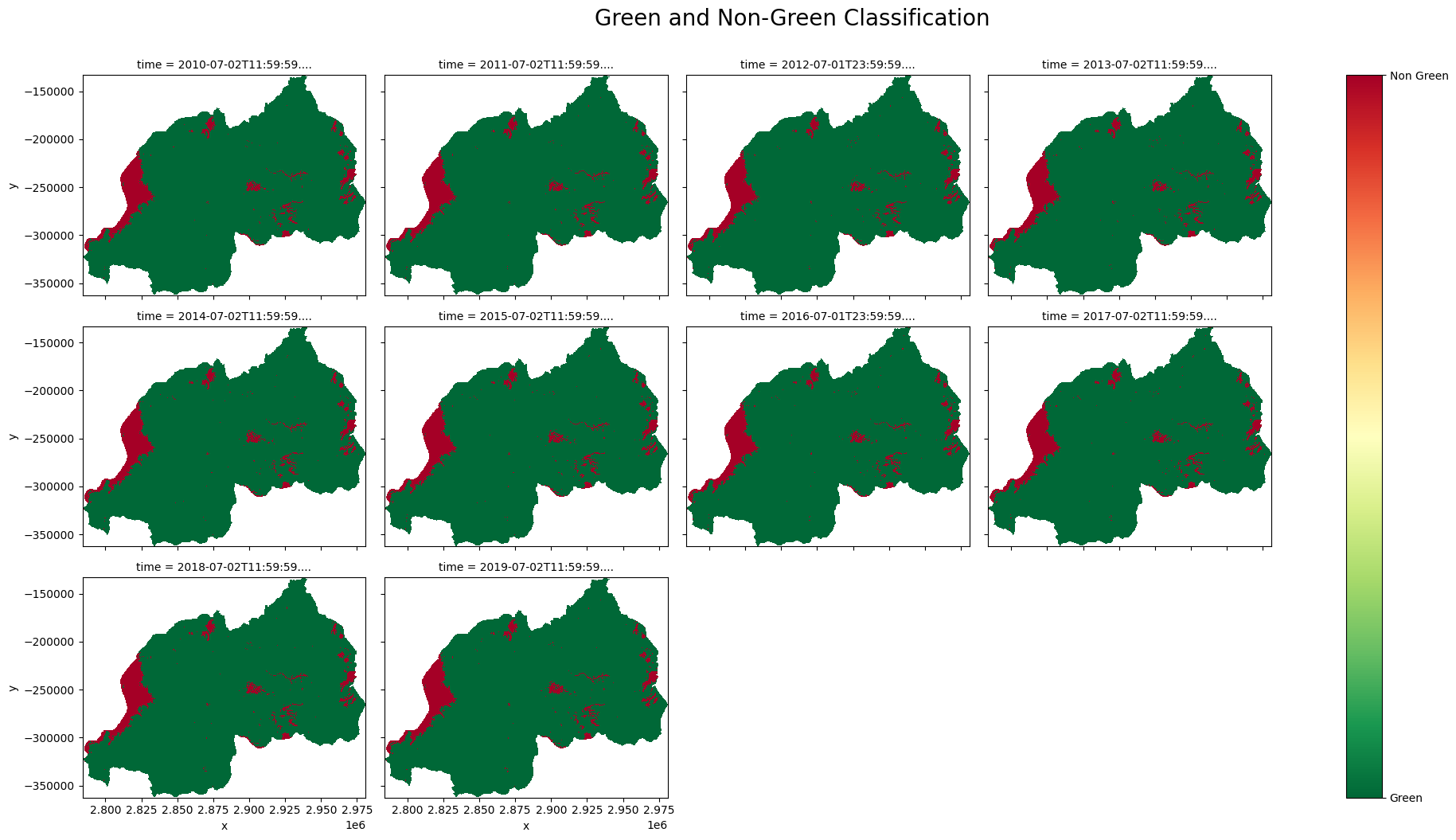
Reclasser la classification du GIEC en classes vertes et non vertes

gng_classess = ["Green", "Non Green"]
gng_classess_num = [1, 2]
recl_condition = [ds_cci["ipcc_classification"].isin([1, 2, 3, 4]),
                  ds_cci["ipcc_classification"].isin([5, 6])]

ds_cci["green_non_green"] = xr.DataArray(np.select(recl_condition, gng_classess_num),
                                         coords={"time": ds_cci.time, "y": ds_cci.y, "x": ds_cci.x},
                                         dims=["time", "y", "x"]).astype("int8").where(mask)

Tracé de la classification verte/non verte

gng = ds_cci["green_non_green"].plot(col='time',
                                     add_colorbar=False,
                                     figsize = (20, 10),
                                     cmap="RdYlGn_r",
                                     col_wrap = 4)


gng.fig.suptitle("Green and Non-Green Classification", ha="center", y=1.05, size=20)
gngp = plt.colorbar(gng._mappables[-1], ax = gng.axs)
gngp.set_ticks(gng_classess_num)
gngp.set_ticklabels(gng_classess)
plt.savefig(f"results/Green_Non_Green_{country}")
plt.show()

Sous-échantillonnage du jeu de données dem_strm à une résolution de 30 à 300 m

ds = (xr_reproject(src=ds, how=ds_cci.odc.geobox)).squeeze()

## Conversion de la surface des pixels

pixel_length = 300  # in metres
m_per_km = 1000  # conversion from metres to kilometres
area_per_pixel = pixel_length ** 2 / m_per_km ** 2

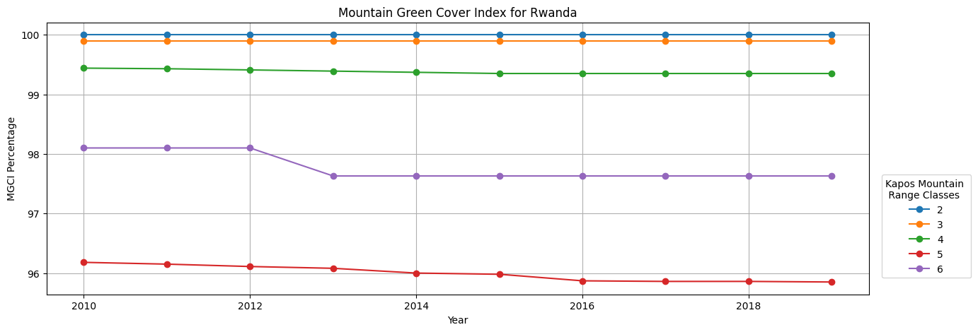
Calcul de l’indice de couverture végétale des montagnes (MGCI)

mgci = {}
years_int=[y[0] for y in ds_cci.groupby('time.year')]
mountain_indices = [y[0] for y in ds.groupby("kapo_class")][1:]

# Mountain Green Cover Area = sum of mountain area (Km2) covered by cropland,
# grassland, forestland, shrubland, and wetland, as defined based on the IPCC classification;
ipcc_green = (ds["kapo_class"].where(ds_cci["ipcc_classification"].isin([1, 2, 3, 4]), np.nan)).astype("int8")

for mountain_index in mountain_indices:
    # Mountain Green Cover Area (Numerator)
    numerator = ipcc_green.where(
        ds['kapo_class'] == mountain_index).sum(dim=["x", "y"])  * area_per_pixel
    # Total Mountain Area = total area (Km2) of mountains. In both the numerator and
    # denominator, Mountain is defined according to Kapos et al. in 2000
    total_mountain_area = ds["kapo_class"].where(
        ds['kapo_class'] == mountain_index).sum(dim=["x", "y"]) * area_per_pixel
    mgci[mountain_index] = (numerator.values / total_mountain_area.values) * 100
mgci = pd.DataFrame.from_dict(mgci, orient="index", columns = years_int)

/opt/venv/lib/python3.12/site-packages/xarray/core/duck_array_ops.py:250: RuntimeWarning: invalid value encountered in cast
  return data.astype(dtype, **kwargs)

mgci = mgci.round(2)

Indice de couverture végétale des montagnes

for n in range(len(mgci)):
    mgci.iloc[n].plot(kind="line", figsize=(15,5), marker='o')

plt.title(f"Mountain Green Cover Index for {country}")
plt.legend(loc='center right', bbox_to_anchor=(1.13, 0.25), title="Kapos Mountain \n Range Classes")
plt.xlabel("Year")
plt.ylabel("MGCI Percentage")
plt.xticks(rotation=0)
plt.grid()
plt.savefig(f"results/MGCI_{country}")
plt.show()

---

Informations Complémentaires

Licence : Le code de ce carnet est sous licence Apache, version 2.0 <https://www.apache.org/licenses/LICENSE-2.0>. Les données de Digital Earth Africa sont sous licence Creative Commons par attribution 4.0 <https://creativecommons.org/licenses/by/4.0/>.

Contact : Si vous avez besoin d’aide, veuillez poster une question sur le canal Slack Open Data Cube <http://slack.opendatacube.org/>`__ ou sur le GIS Stack Exchange en utilisant la balise open-data-cube (vous pouvez consulter les questions posées précédemment ici). Si vous souhaitez signaler un problème avec ce bloc-notes, vous pouvez en déposer un sur Github.

Version de Datacube compatible :

print(datacube.__version__)

1.9.13

Dernier test :

from datetime import datetime
datetime.today().strftime('%Y-%m-%d')

'2026-04-13'